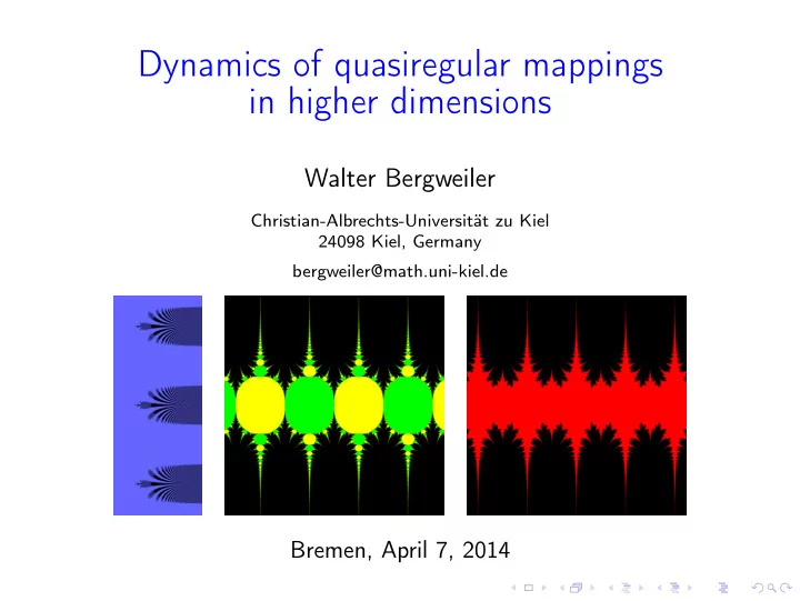
Dynamics of quasiregular mappings in higher dimensions Walter - - PowerPoint PPT Presentation

Dynamics of quasiregular mappings in higher dimensions

Walter Bergweiler

Christian-Albrechts-Universität zu Kiel 24098 Kiel, Germany bergweiler@math.uni-kiel.de

Bremen, April 7, 2014

Iteration of exponential functions Eλ(z) = λez

2

Iteration of exponential functions Eλ(z) = λez

2

f : C → C entire, f n = f ◦ f ◦ · · · ◦ f

Iteration of exponential functions Eλ(z) = λez

2

f : C → C entire, f n = f ◦ f ◦ · · · ◦ f Julia set: J(f ) = {z ∈ C: {f n} not normal in z}

Iteration of exponential functions Eλ(z) = λez

2

f : C → C entire, f n = f ◦ f ◦ · · · ◦ f Julia set: J(f ) = {z ∈ C: {f n} not normal in z} Attracting fixed point ξ: f (ξ) = ξ and |f ′(ξ)| < 1

Iteration of exponential functions Eλ(z) = λez

2

f : C → C entire, f n = f ◦ f ◦ · · · ◦ f Julia set: J(f ) = {z ∈ C: {f n} not normal in z} Attracting fixed point ξ: f (ξ) = ξ and |f ′(ξ)| < 1 Basin of attraction: A(ξ) = {z ∈ C: f n(z) → ξ}

Iteration of exponential functions Eλ(z) = λez

2

f : C → C entire, f n = f ◦ f ◦ · · · ◦ f Julia set: J(f ) = {z ∈ C: {f n} not normal in z} Attracting fixed point ξ: f (ξ) = ξ and |f ′(ξ)| < 1 Basin of attraction: A(ξ) = {z ∈ C: f n(z) → ξ} Fact: J(f ) = ∂A(ξ)

Iteration of exponential functions Eλ(z) = λez

2

f : C → C entire, f n = f ◦ f ◦ · · · ◦ f Julia set: J(f ) = {z ∈ C: {f n} not normal in z} Attracting fixed point ξ: f (ξ) = ξ and |f ′(ξ)| < 1 Basin of attraction: A(ξ) = {z ∈ C: f n(z) → ξ} Fact: J(f ) = ∂A(ξ) Consider Eλ(z) = λez where 0 < λ < 1

e

Iteration of exponential functions Eλ(z) = λez

2

f : C → C entire, f n = f ◦ f ◦ · · · ◦ f Julia set: J(f ) = {z ∈ C: {f n} not normal in z} Attracting fixed point ξ: f (ξ) = ξ and |f ′(ξ)| < 1 Basin of attraction: A(ξ) = {z ∈ C: f n(z) → ξ} Fact: J(f ) = ∂A(ξ) Consider Eλ(z) = λez where 0 < λ < 1

e

Eλ has an attracting fixed point ξ

Iteration of exponential functions Eλ(z) = λez

2

f : C → C entire, f n = f ◦ f ◦ · · · ◦ f Julia set: J(f ) = {z ∈ C: {f n} not normal in z} Attracting fixed point ξ: f (ξ) = ξ and |f ′(ξ)| < 1 Basin of attraction: A(ξ) = {z ∈ C: f n(z) → ξ} Fact: J(f ) = ∂A(ξ) Consider Eλ(z) = λez where 0 < λ < 1

e

Eλ has an attracting fixed point ξ

Iteration of exponential functions Eλ(z) = λez

2

f : C → C entire, f n = f ◦ f ◦ · · · ◦ f Julia set: J(f ) = {z ∈ C: {f n} not normal in z} Attracting fixed point ξ: f (ξ) = ξ and |f ′(ξ)| < 1 Basin of attraction: A(ξ) = {z ∈ C: f n(z) → ξ} Fact: J(f ) = ∂A(ξ) Consider Eλ(z) = λez where 0 < λ < 1

e

Eλ has an attracting fixed point ξ Devaney-Krych 1984: J(Eλ) = C\A(ξ) and J(Eλ) is a “Cantor set of curves”.

Iteration of exponential functions Eλ(z) = λez

3

Iteration of exponential functions Eλ(z) = λez

4

Let γ : [0, ∞) → C be an injective curve with limt→∞ γ(t) = ∞.

Iteration of exponential functions Eλ(z) = λez

4

Let γ : [0, ∞) → C be an injective curve with limt→∞ γ(t) = ∞. Then γ([0, ∞)) is called a hair and γ(0) is called the endpoint.

Iteration of exponential functions Eλ(z) = λez

4

Let γ : [0, ∞) → C be an injective curve with limt→∞ γ(t) = ∞. Then γ([0, ∞)) is called a hair and γ(0) is called the endpoint. Devaney-Krych 1984: J(Eλ) is an uncountable union of pairwise disjoint hairs.

Iteration of exponential functions Eλ(z) = λez

4

Let γ : [0, ∞) → C be an injective curve with limt→∞ γ(t) = ∞. Then γ([0, ∞)) is called a hair and γ(0) is called the endpoint. Devaney-Krych 1984: J(Eλ) is an uncountable union of pairwise disjoint hairs. Idea of proof: partition C into strips of width 2π.

Iteration of exponential functions Eλ(z) = λez

4

Let γ : [0, ∞) → C be an injective curve with limt→∞ γ(t) = ∞. Then γ([0, ∞)) is called a hair and γ(0) is called the endpoint. Devaney-Krych 1984: J(Eλ) is an uncountable union of pairwise disjoint hairs. Idea of proof: partition C into strips of width 2π. z, w equivalent :⇔ E k

λ (z) and E k λ (w) in same strip for all k.

Iteration of exponential functions Eλ(z) = λez

4

Let γ : [0, ∞) → C be an injective curve with limt→∞ γ(t) = ∞. Then γ([0, ∞)) is called a hair and γ(0) is called the endpoint. Devaney-Krych 1984: J(Eλ) is an uncountable union of pairwise disjoint hairs. Idea of proof: partition C into strips of width 2π. z, w equivalent :⇔ E k

λ (z) and E k λ (w) in same strip for all k.

Show that equivalence classes are hairs.

Iteration of exponential functions Eλ(z) = λez

4

Let γ : [0, ∞) → C be an injective curve with limt→∞ γ(t) = ∞. Then γ([0, ∞)) is called a hair and γ(0) is called the endpoint. Devaney-Krych 1984: J(Eλ) is an uncountable union of pairwise disjoint hairs. Idea of proof: partition C into strips of width 2π. z, w equivalent :⇔ E k

λ (z) and E k λ (w) in same strip for all k.

Show that equivalence classes are hairs. Let dim A be the Hausdorff dimension of a set A.

Iteration of exponential functions Eλ(z) = λez

4

Let γ : [0, ∞) → C be an injective curve with limt→∞ γ(t) = ∞. Then γ([0, ∞)) is called a hair and γ(0) is called the endpoint. Devaney-Krych 1984: J(Eλ) is an uncountable union of pairwise disjoint hairs. Idea of proof: partition C into strips of width 2π. z, w equivalent :⇔ E k

λ (z) and E k λ (w) in same strip for all k.

Show that equivalence classes are hairs. Let dim A be the Hausdorff dimension of a set A. This means that dim A is the infimum of all s > 0 for which lim

δ→0 inf Aj

  

∞

• j=1

(diam Aj)s : A ⊂

∞

• j=1

Aj, diam Aj < δ    < ∞.

Iteration of exponential functions Eλ(z) = λez

4

Let γ : [0, ∞) → C be an injective curve with limt→∞ γ(t) = ∞. Then γ([0, ∞)) is called a hair and γ(0) is called the endpoint. Devaney-Krych 1984: J(Eλ) is an uncountable union of pairwise disjoint hairs. Idea of proof: partition C into strips of width 2π. z, w equivalent :⇔ E k

λ (z) and E k λ (w) in same strip for all k.

Show that equivalence classes are hairs. Let dim A be the Hausdorff dimension of a set A. This means that dim A is the infimum of all s > 0 for which lim

δ→0 inf Aj

  

∞

• j=1

(diam Aj)s : A ⊂

∞

• j=1

Aj, diam Aj < δ    < ∞. McMullen 1987: dim J(Eλ) = 2, but area J(Eλ) = 0.

Iteration of exponential functions Eλ(z) = λez

4

Let γ : [0, ∞) → C be an injective curve with limt→∞ γ(t) = ∞. Then γ([0, ∞)) is called a hair and γ(0) is called the endpoint. Devaney-Krych 1984: J(Eλ) is an uncountable union of pairwise disjoint hairs. Idea of proof: partition C into strips of width 2π. z, w equivalent :⇔ E k

λ (z) and E k λ (w) in same strip for all k.

Show that equivalence classes are hairs. Let dim A be the Hausdorff dimension of a set A. This means that dim A is the infimum of all s > 0 for which lim

δ→0 inf Aj

  

∞

• j=1

(diam Aj)s : A ⊂

∞

• j=1

Aj, diam Aj < δ    < ∞. McMullen 1987: dim J(Eλ) = 2, but area J(Eλ) = 0. Let Xλ be the set of endpoints of the hairs in J(Eλ).

Iteration of exponential functions Eλ(z) = λez

4

Let γ : [0, ∞) → C be an injective curve with limt→∞ γ(t) = ∞. Then γ([0, ∞)) is called a hair and γ(0) is called the endpoint. Devaney-Krych 1984: J(Eλ) is an uncountable union of pairwise disjoint hairs. Idea of proof: partition C into strips of width 2π. z, w equivalent :⇔ E k

λ (z) and E k λ (w) in same strip for all k.

Show that equivalence classes are hairs. Let dim A be the Hausdorff dimension of a set A. This means that dim A is the infimum of all s > 0 for which lim

δ→0 inf Aj

  

∞

• j=1

(diam Aj)s : A ⊂

∞

• j=1

Aj, diam Aj < δ    < ∞. McMullen 1987: dim J(Eλ) = 2, but area J(Eλ) = 0. Let Xλ be the set of endpoints of the hairs in J(Eλ). Karpińska 1999: dim Xλ = 2 and dim(J(Eλ)\Xλ) = 1.

Trigonometric functions Tλ,µ(z) = sin(λz + µ)

5

Trigonometric functions Tλ,µ(z) = sin(λz + µ)

5

Devaney-Tangerman 1984: 0 < λ < 1 , µ = 0 ⇒ J(Tλ,µ) is an uncountable union of pairwise disjoint hairs.

Trigonometric functions Tλ,µ(z) = sin(λz + µ)

5

Devaney-Tangerman 1984: 0 < λ < 1 , µ = 0 ⇒ J(Tλ,µ) is an uncountable union of pairwise disjoint hairs. McMullen 1987: λ = 0 ⇒ area J(Tλ,µ) > 0.

Trigonometric functions Tλ,µ(z) = sin(λz + µ)

5

Devaney-Tangerman 1984: 0 < λ < 1 , µ = 0 ⇒ J(Tλ,µ) is an uncountable union of pairwise disjoint hairs. McMullen 1987: λ = 0 ⇒ area J(Tλ,µ) > 0. 0 < λ < 1, µ = 0, X = set of endpoints of the hairs

Trigonometric functions Tλ,µ(z) = sin(λz + µ)

5

Devaney-Tangerman 1984: 0 < λ < 1 , µ = 0 ⇒ J(Tλ,µ) is an uncountable union of pairwise disjoint hairs. McMullen 1987: λ = 0 ⇒ area J(Tλ,µ) > 0. 0 < λ < 1, µ = 0, X = set of endpoints of the hairs Karpińska 1999: area X > 0 (and dim(J(Tλ,µ)\X) = 1).

Trigonometric functions Tλ,µ(z) = sin(λz + µ)

5

Devaney-Tangerman 1984: 0 < λ < 1 , µ = 0 ⇒ J(Tλ,µ) is an uncountable union of pairwise disjoint hairs. McMullen 1987: λ = 0 ⇒ area J(Tλ,µ) > 0. 0 < λ < 1, µ = 0, X = set of endpoints of the hairs Karpińska 1999: area X > 0 (and dim(J(Tλ,µ)\X) = 1). Fact: If λ, µ are such that the critical values of Tλ,µ are preperiodic, then J(Tλ,µ) = C.

Trigonometric functions Tλ,µ(z) = sin(λz + µ)

5

Devaney-Tangerman 1984: 0 < λ < 1 , µ = 0 ⇒ J(Tλ,µ) is an uncountable union of pairwise disjoint hairs. McMullen 1987: λ = 0 ⇒ area J(Tλ,µ) > 0. 0 < λ < 1, µ = 0, X = set of endpoints of the hairs Karpińska 1999: area X > 0 (and dim(J(Tλ,µ)\X) = 1). Fact: If λ, µ are such that the critical values of Tλ,µ are preperiodic, then J(Tλ,µ) = C. For example f (z) = sin πz.

Trigonometric functions Tλ,µ(z) = sin(λz + µ)

5

Devaney-Tangerman 1984: 0 < λ < 1 , µ = 0 ⇒ J(Tλ,µ) is an uncountable union of pairwise disjoint hairs. McMullen 1987: λ = 0 ⇒ area J(Tλ,µ) > 0. 0 < λ < 1, µ = 0, X = set of endpoints of the hairs Karpińska 1999: area X > 0 (and dim(J(Tλ,µ)\X) = 1). Fact: If λ, µ are such that the critical values of Tλ,µ are preperiodic, then J(Tλ,µ) = C. For example f (z) = sin πz. Schleicher 2007: For such λ, µ the Julia set C is still union of

• hairs. The hairs may intersect only in their endpoints. Moreover,

dim(C\X) = 1. In particular, area(C\X) = 0.

Trigonometric functions Tλ,µ(z) = sin(λz + µ)

5

Devaney-Tangerman 1984: 0 < λ < 1 , µ = 0 ⇒ J(Tλ,µ) is an uncountable union of pairwise disjoint hairs. McMullen 1987: λ = 0 ⇒ area J(Tλ,µ) > 0. 0 < λ < 1, µ = 0, X = set of endpoints of the hairs Karpińska 1999: area X > 0 (and dim(J(Tλ,µ)\X) = 1). Fact: If λ, µ are such that the critical values of Tλ,µ are preperiodic, then J(Tλ,µ) = C. For example f (z) = sin πz. Schleicher 2007: For such λ, µ the Julia set C is still union of

• hairs. The hairs may intersect only in their endpoints. Moreover,

dim(C\X) = 1. In particular, area(C\X) = 0. Forget complex dynamics.

Trigonometric functions Tλ,µ(z) = sin(λz + µ)

5

Devaney-Tangerman 1984: 0 < λ < 1 , µ = 0 ⇒ J(Tλ,µ) is an uncountable union of pairwise disjoint hairs. McMullen 1987: λ = 0 ⇒ area J(Tλ,µ) > 0. 0 < λ < 1, µ = 0, X = set of endpoints of the hairs Karpińska 1999: area X > 0 (and dim(J(Tλ,µ)\X) = 1). Fact: If λ, µ are such that the critical values of Tλ,µ are preperiodic, then J(Tλ,µ) = C. For example f (z) = sin πz. Schleicher 2007: For such λ, µ the Julia set C is still union of

• hairs. The hairs may intersect only in their endpoints. Moreover,

dim(C\X) = 1. In particular, area(C\X) = 0. Forget complex dynamics. Schleicher’s result says:

Trigonometric functions Tλ,µ(z) = sin(λz + µ)

5

Devaney-Tangerman 1984: 0 < λ < 1 , µ = 0 ⇒ J(Tλ,µ) is an uncountable union of pairwise disjoint hairs. McMullen 1987: λ = 0 ⇒ area J(Tλ,µ) > 0. 0 < λ < 1, µ = 0, X = set of endpoints of the hairs Karpińska 1999: area X > 0 (and dim(J(Tλ,µ)\X) = 1). Fact: If λ, µ are such that the critical values of Tλ,µ are preperiodic, then J(Tλ,µ) = C. For example f (z) = sin πz. Schleicher 2007: For such λ, µ the Julia set C is still union of

• hairs. The hairs may intersect only in their endpoints. Moreover,

dim(C\X) = 1. In particular, area(C\X) = 0. Forget complex dynamics. Schleicher’s result says: There exists a partition of the plane in sets X and Y , with Y of measure zero, such that Y consists of disjoint, open injective curves connecting a point in X with ∞, and every point of X is the endpoint of at least one curve in Y .

Exponential and trigonometric functions in R3

6

Exponential and trigonometric functions in R3

6

A way to define the complex exponential function (if the real exponential function is known):

Exponential and trigonometric functions in R3

6

A way to define the complex exponential function (if the real exponential function is known): Start with map ϕ from segment

• −π

2 i, π 2 i

• to half circle

{z ∈ C: |z| = 1, Re z ≥ 0}. (Take ϕ(t) = cos t + i sin t.) Put S = {z ∈ C: |Im z| ≤ π

2 } and define E : S → {z : Re z > 0}

by E(x + iy) = exϕ(y).

Exponential and trigonometric functions in R3

6

A way to define the complex exponential function (if the real exponential function is known): Start with map ϕ from segment

• −π

2 i, π 2 i

• to half circle

{z ∈ C: |z| = 1, Re z ≥ 0}. (Take ϕ(t) = cos t + i sin t.) Put S = {z ∈ C: |Im z| ≤ π

2 } and define E : S → {z : Re z > 0}

by E(x + iy) = exϕ(y).

Exponential and trigonometric functions in R3

6

A way to define the complex exponential function (if the real exponential function is known): Start with map ϕ from segment

• −π

2 i, π 2 i

• to half circle

{z ∈ C: |z| = 1, Re z ≥ 0}. (Take ϕ(t) = cos t + i sin t.) Put S = {z ∈ C: |Im z| ≤ π

2 } and H = {z : Re z > 0}.

Define E : S → H by E(x + iy) = exϕ(y).

Exponential and trigonometric functions in R3

6

A way to define the complex exponential function (if the real exponential function is known): Start with map ϕ from segment

• −π

2 i, π 2 i

• to half circle

{z ∈ C: |z| = 1, Re z ≥ 0}. (Take ϕ(t) = cos t + i sin t.) Put S = {z ∈ C: |Im z| ≤ π

2 } and H = {z : Re z > 0}.

Define E : S → H by E(x + iy) = exϕ(y).

Exponential and trigonometric functions in R3

6

A way to define the complex exponential function (if the real exponential function is known): Start with map ϕ from segment

• −π

2 i, π 2 i

• to half circle

{z ∈ C: |z| = 1, Re z ≥ 0}. (Take ϕ(t) = cos t + i sin t.) Put S = {z ∈ C: |Im z| ≤ π

2 } and H = {z : Re z > 0}.

Define E : S → H by E(x + iy) = exϕ(y).

Exponential and trigonometric functions in R3

6

A way to define the complex exponential function (if the real exponential function is known): Start with map ϕ from segment

• −π

2 i, π 2 i

• to half circle

{z ∈ C: |z| = 1, Re z ≥ 0}. (Take ϕ(t) = cos t + i sin t.) Put S = {z ∈ C: |Im z| ≤ π

2 } and H = {z : Re z > 0}.

Define E : S → H by E(x + iy) = exϕ(y).

Exponential and trigonometric functions in R3

6

A way to define the complex exponential function (if the real exponential function is known): Start with map ϕ from segment

• −π

2 i, π 2 i

• to half circle

{z ∈ C: |z| = 1, Re z ≥ 0}. (Take ϕ(t) = cos t + i sin t.) Put S = {z ∈ C: |Im z| ≤ π

2 } and H = {z : Re z > 0}.

Define E : S → H by E(x + iy) = exϕ(y). Extend E : S → H to a map from E : C → C by reflection.

Exponential and trigonometric functions in R3

7

Exponential and trigonometric functions in R3

7

Analogue in dimension 3 (Zorich 1969; also Iwaniec/Martin 2001):

Exponential and trigonometric functions in R3

7

Analogue in dimension 3 (Zorich 1969; also Iwaniec/Martin 2001): Map square Q = {(x, y) ∈ R2 : |x| ≤ 1, |y| ≤ 1} to hemisphere {(x, y, z) ∈ R3 : x2 + y2 + z2 = 1, z ≥ 0} by (bilipschitz) map ϕ.

Exponential and trigonometric functions in R3

7

Analogue in dimension 3 (Zorich 1969; also Iwaniec/Martin 2001): Map square Q = {(x, y) ∈ R2 : |x| ≤ 1, |y| ≤ 1} to hemisphere {(x, y, z) ∈ R3 : x2 + y2 + z2 = 1, z ≥ 0} by (bilipschitz) map ϕ.

Exponential and trigonometric functions in R3

7

Analogue in dimension 3 (Zorich 1969; also Iwaniec/Martin 2001): Map square Q = {(x, y) ∈ R2 : |x| ≤ 1, |y| ≤ 1} to hemisphere {(x, y, z) ∈ R3 : x2 + y2 + z2 = 1, z ≥ 0} by (bilipschitz) map ϕ. Define F : Q × R → R3 by F(x, y, z) = ezϕ(x, y). Then F maps a “square beam” to a half-space.

Exponential and trigonometric functions in R3

7

Analogue in dimension 3 (Zorich 1969; also Iwaniec/Martin 2001): Map square Q = {(x, y) ∈ R2 : |x| ≤ 1, |y| ≤ 1} to hemisphere {(x, y, z) ∈ R3 : x2 + y2 + z2 = 1, z ≥ 0} by (bilipschitz) map ϕ. Define F : Q × R → R3 by F(x, y, z) = ezϕ(x, y). Then F maps a “square beam” to a half-space.

Exponential and trigonometric functions in R3

7

Analogue in dimension 3 (Zorich 1969; also Iwaniec/Martin 2001): Map square Q = {(x, y) ∈ R2 : |x| ≤ 1, |y| ≤ 1} to hemisphere {(x, y, z) ∈ R3 : x2 + y2 + z2 = 1, z ≥ 0} by (bilipschitz) map ϕ. Define F : Q × R → R3 by F(x, y, z) = ezϕ(x, y). Then F maps a “square beam” to a half-space.

Exponential and trigonometric functions in R3

7

Analogue in dimension 3 (Zorich 1969; also Iwaniec/Martin 2001): Map square Q = {(x, y) ∈ R2 : |x| ≤ 1, |y| ≤ 1} to hemisphere {(x, y, z) ∈ R3 : x2 + y2 + z2 = 1, z ≥ 0} by (bilipschitz) map ϕ. Define F : Q × R → R3 by F(x, y, z) = ezϕ(x, y). Then F maps a “square beam” to a half-space.

Exponential and trigonometric functions in R3

7

Analogue in dimension 3 (Zorich 1969; also Iwaniec/Martin 2001): Map square Q = {(x, y) ∈ R2 : |x| ≤ 1, |y| ≤ 1} to hemisphere {(x, y, z) ∈ R3 : x2 + y2 + z2 = 1, z ≥ 0} by (bilipschitz) map ϕ. Define F : Q × R → R3 by F(x, y, z) = ezϕ(x, y). Then F maps a “square beam” to a half-space.

Exponential and trigonometric functions in R3

7

Analogue in dimension 3 (Zorich 1969; also Iwaniec/Martin 2001): Map square Q = {(x, y) ∈ R2 : |x| ≤ 1, |y| ≤ 1} to hemisphere {(x, y, z) ∈ R3 : x2 + y2 + z2 = 1, z ≥ 0} by (bilipschitz) map ϕ. Define F : Q × R → R3 by F(x, y, z) = ezϕ(x, y). Then F maps a “square beam” to a half-space.

Exponential and trigonometric functions in R3

7

Analogue in dimension 3 (Zorich 1969; also Iwaniec/Martin 2001): Map square Q = {(x, y) ∈ R2 : |x| ≤ 1, |y| ≤ 1} to hemisphere {(x, y, z) ∈ R3 : x2 + y2 + z2 = 1, z ≥ 0} by (bilipschitz) map ϕ. Define F : Q × R → R3 by F(x, y, z) = ezϕ(x, y). Then F maps a “square beam” to a half-space. Extend F to a map from R3 to R3 by reflection.

Exponential and trigonometric functions in R3

7

Analogue in dimension 3 (Zorich 1969; also Iwaniec/Martin 2001): Map square Q = {(x, y) ∈ R2 : |x| ≤ 1, |y| ≤ 1} to hemisphere {(x, y, z) ∈ R3 : x2 + y2 + z2 = 1, z ≥ 0} by (bilipschitz) map ϕ. Define F : Q × R → R3 by F(x, y, z) = ezϕ(x, y). Then F maps a “square beam” to a half-space. Extend F to a map from R3 to R3 by reflection. The map F is called Zorich map.

Exponential and trigonometric functions in R3

7

Analogue in dimension 3 (Zorich 1969; also Iwaniec/Martin 2001): Map square Q = {(x, y) ∈ R2 : |x| ≤ 1, |y| ≤ 1} to hemisphere {(x, y, z) ∈ R3 : x2 + y2 + z2 = 1, z ≥ 0} by (bilipschitz) map ϕ. Define F : Q × R → R3 by F(x, y, z) = ezϕ(x, y). Then F maps a “square beam” to a half-space. Extend F to a map from R3 to R3 by reflection. The map F is called Zorich map. Similarly: analogues T : R3 → R3 of sine and cosine:

Exponential and trigonometric functions in R3

7

Analogue in dimension 3 (Zorich 1969; also Iwaniec/Martin 2001): Map square Q = {(x, y) ∈ R2 : |x| ≤ 1, |y| ≤ 1} to hemisphere {(x, y, z) ∈ R3 : x2 + y2 + z2 = 1, z ≥ 0} by (bilipschitz) map ϕ. Define F : Q × R → R3 by F(x, y, z) = ezϕ(x, y). Then F maps a “square beam” to a half-space. Extend F to a map from R3 to R3 by reflection. The map F is called Zorich map. Similarly: analogues T : R3 → R3 of sine and cosine: Replace beam Q × R by half-beam Q × {x ∈ R: x ≥ 0}.

Exponential and trigonometric functions in R3

7

Analogue in dimension 3 (Zorich 1969; also Iwaniec/Martin 2001): Map square Q = {(x, y) ∈ R2 : |x| ≤ 1, |y| ≤ 1} to hemisphere {(x, y, z) ∈ R3 : x2 + y2 + z2 = 1, z ≥ 0} by (bilipschitz) map ϕ. Define F : Q × R → R3 by F(x, y, z) = ezϕ(x, y). Then F maps a “square beam” to a half-space. Extend F to a map from R3 to R3 by reflection. The map F is called Zorich map. Similarly: analogues T : R3 → R3 of sine and cosine: Replace beam Q × R by half-beam Q × {x ∈ R: x ≥ 0}. Construct map T from half-beam to half-space.

Iteration in R3

8

Iteration in R3

8

Consider Fa(x1, x2, x3)=F(x1, x2, x3)−(0, 0, a) with Zorich map F.

Iteration in R3

8

Consider Fa(x1, x2, x3)=F(x1, x2, x3)−(0, 0, a) with Zorich map F.

• B. 2010: For large a the function Fa has an attracting fixed point

ξ such that

◮ {x : f n(x)→ξ} is uncountable union of pairwise disjoint hairs, ◮ the endpoints of the hairs have Hausdorff dimension 3, ◮ the hairs without endpoints have Hausdorff dimension 1.

Iteration in R3

8

Consider Fa(x1, x2, x3)=F(x1, x2, x3)−(0, 0, a) with Zorich map F.

• B. 2010: For large a the function Fa has an attracting fixed point

ξ such that

◮ {x : f n(x)→ξ} is uncountable union of pairwise disjoint hairs, ◮ the endpoints of the hairs have Hausdorff dimension 3, ◮ the hairs without endpoints have Hausdorff dimension 1.

Let Tλ = λT with T generalized cosine and λ > 0.

Iteration in R3

8

Consider Fa(x1, x2, x3)=F(x1, x2, x3)−(0, 0, a) with Zorich map F.

• B. 2010: For large a the function Fa has an attracting fixed point

ξ such that

◮ {x : f n(x)→ξ} is uncountable union of pairwise disjoint hairs, ◮ the endpoints of the hairs have Hausdorff dimension 3, ◮ the hairs without endpoints have Hausdorff dimension 1.

Let Tλ = λT with T generalized cosine and λ > 0. Consider natural decomposition of R3 into “half-beams”.

Iteration in R3

8

Consider Fa(x1, x2, x3)=F(x1, x2, x3)−(0, 0, a) with Zorich map F.

• B. 2010: For large a the function Fa has an attracting fixed point

ξ such that

◮ {x : f n(x)→ξ} is uncountable union of pairwise disjoint hairs, ◮ the endpoints of the hairs have Hausdorff dimension 3, ◮ the hairs without endpoints have Hausdorff dimension 1.

Let Tλ = λT with T generalized cosine and λ > 0. Consider natural decomposition of R3 into “half-beams”. x, y equivalent :⇔ T k

λ (x) and T k λ (y) in same half-beam for all k.

Iteration in R3

8

Consider Fa(x1, x2, x3)=F(x1, x2, x3)−(0, 0, a) with Zorich map F.

• B. 2010: For large a the function Fa has an attracting fixed point

ξ such that

◮ {x : f n(x)→ξ} is uncountable union of pairwise disjoint hairs, ◮ the endpoints of the hairs have Hausdorff dimension 3, ◮ the hairs without endpoints have Hausdorff dimension 1.

Let Tλ = λT with T generalized cosine and λ > 0. Consider natural decomposition of R3 into “half-beams”. x, y equivalent :⇔ T k

λ (x) and T k λ (y) in same half-beam for all k.

Eremenko, B. 2011: For large λ, the equivalence classes are

• hairs. Two hairs can intersect only in their endpoints. The union of

hairs without endpoints has Hausdorff dimension 1.

Iteration in R3

8

Consider Fa(x1, x2, x3)=F(x1, x2, x3)−(0, 0, a) with Zorich map F.

• B. 2010: For large a the function Fa has an attracting fixed point

ξ such that

◮ {x : f n(x)→ξ} is uncountable union of pairwise disjoint hairs, ◮ the endpoints of the hairs have Hausdorff dimension 3, ◮ the hairs without endpoints have Hausdorff dimension 1.

Let Tλ = λT with T generalized cosine and λ > 0. Consider natural decomposition of R3 into “half-beams”. x, y equivalent :⇔ T k

λ (x) and T k λ (y) in same half-beam for all k.

Eremenko, B. 2011: For large λ, the equivalence classes are

• hairs. Two hairs can intersect only in their endpoints. The union of

hairs without endpoints has Hausdorff dimension 1. Obtain paradoxical situation described before in R3

Iteration in R3

8

Consider Fa(x1, x2, x3)=F(x1, x2, x3)−(0, 0, a) with Zorich map F.

• B. 2010: For large a the function Fa has an attracting fixed point

ξ such that

◮ {x : f n(x)→ξ} is uncountable union of pairwise disjoint hairs, ◮ the endpoints of the hairs have Hausdorff dimension 3, ◮ the hairs without endpoints have Hausdorff dimension 1.

Let Tλ = λT with T generalized cosine and λ > 0. Consider natural decomposition of R3 into “half-beams”. x, y equivalent :⇔ T k

λ (x) and T k λ (y) in same half-beam for all k.

Eremenko, B. 2011: For large λ, the equivalence classes are

• hairs. Two hairs can intersect only in their endpoints. The union of

hairs without endpoints has Hausdorff dimension 1. Obtain paradoxical situation described before in R3, in fact in Rd.

Iteration in R3

8

Consider Fa(x1, x2, x3)=F(x1, x2, x3)−(0, 0, a) with Zorich map F.

• B. 2010: For large a the function Fa has an attracting fixed point

ξ such that

◮ {x : f n(x)→ξ} is uncountable union of pairwise disjoint hairs, ◮ the endpoints of the hairs have Hausdorff dimension 3, ◮ the hairs without endpoints have Hausdorff dimension 1.

Let Tλ = λT with T generalized cosine and λ > 0. Consider natural decomposition of R3 into “half-beams”. x, y equivalent :⇔ T k

λ (x) and T k λ (y) in same half-beam for all k.

Eremenko, B. 2011: For large λ, the equivalence classes are

• hairs. Two hairs can intersect only in their endpoints. The union of

hairs without endpoints has Hausdorff dimension 1. Obtain paradoxical situation described before in R3, in fact in Rd. Even more paradox:

Iteration in R3

8

Consider Fa(x1, x2, x3)=F(x1, x2, x3)−(0, 0, a) with Zorich map F.

• B. 2010: For large a the function Fa has an attracting fixed point

ξ such that

◮ {x : f n(x)→ξ} is uncountable union of pairwise disjoint hairs, ◮ the endpoints of the hairs have Hausdorff dimension 3, ◮ the hairs without endpoints have Hausdorff dimension 1.

Let Tλ = λT with T generalized cosine and λ > 0. Consider natural decomposition of R3 into “half-beams”. x, y equivalent :⇔ T k

λ (x) and T k λ (y) in same half-beam for all k.

Eremenko, B. 2011: For large λ, the equivalence classes are

• hairs. Two hairs can intersect only in their endpoints. The union of

hairs without endpoints has Hausdorff dimension 1. Obtain paradoxical situation described before in R3, in fact in Rd. Even more paradox: proof is easier than in C.

Quasiregular maps

9

Quasiregular maps

9

Zorich’s map and the analogues of the trigonometric functions are quasiregular maps from R3 to R3.

Quasiregular maps

9

Zorich’s map and the analogues of the trigonometric functions are quasiregular maps from R3 to R3. Let Ω ⊂ Rd open, f : Ω → Rd continuous.

Quasiregular maps

9

Zorich’s map and the analogues of the trigonometric functions are quasiregular maps from R3 to R3. Let Ω ⊂ Rd open, f : Ω → Rd continuous. Then f is called quasiregular if

Quasiregular maps

9

Zorich’s map and the analogues of the trigonometric functions are quasiregular maps from R3 to R3. Let Ω ⊂ Rd open, f : Ω → Rd continuous. Then f is called quasiregular if

• 1. f ∈ W 1,d

loc (Ω)

Quasiregular maps

9

Zorich’s map and the analogues of the trigonometric functions are quasiregular maps from R3 to R3. Let Ω ⊂ Rd open, f : Ω → Rd continuous. Then f is called quasiregular if

• 1. f ∈ W 1,d

loc (Ω)

(equivalently: f is absolutely continuous on almost all lines parallel to the coordinate axes, with first partial derivatives locally in Ld),

Quasiregular maps

9

Zorich’s map and the analogues of the trigonometric functions are quasiregular maps from R3 to R3. Let Ω ⊂ Rd open, f : Ω → Rd continuous. Then f is called quasiregular if

• 1. f ∈ W 1,d

loc (Ω)

(equivalently: f is absolutely continuous on almost all lines parallel to the coordinate axes, with first partial derivatives locally in Ld),

• 2. there exists K ≥ 1 such that |Df (x)|d ≤ KJf (x) almost

everywhere.

Quasiregular maps

9

Zorich’s map and the analogues of the trigonometric functions are quasiregular maps from R3 to R3. Let Ω ⊂ Rd open, f : Ω → Rd continuous. Then f is called quasiregular if

• 1. f ∈ W 1,d

loc (Ω)

(equivalently: f is absolutely continuous on almost all lines parallel to the coordinate axes, with first partial derivatives locally in Ld),

• 2. there exists K ≥ 1 such that |Df (x)|d ≤ KJf (x) almost

everywhere. Here Df is the derivative and Jf the Jacobian determinant.

Quasiregular maps

9

Zorich’s map and the analogues of the trigonometric functions are quasiregular maps from R3 to R3. Let Ω ⊂ Rd open, f : Ω → Rd continuous. Then f is called quasiregular if

• 1. f ∈ W 1,d

loc (Ω)

(equivalently: f is absolutely continuous on almost all lines parallel to the coordinate axes, with first partial derivatives locally in Ld),

• 2. there exists K ≥ 1 such that |Df (x)|d ≤ KJf (x) almost

everywhere. Here Df is the derivative and Jf the Jacobian determinant. Idea: infinitesimal balls are mapped to infinitesimal ellipsoids, with ratios of semiaxes of these ellipsoids bounded (almost everywhere).

Quasiregular maps

9

Zorich’s map and the analogues of the trigonometric functions are quasiregular maps from R3 to R3. Let Ω ⊂ Rd open, f : Ω → Rd continuous. Then f is called quasiregular if

• 1. f ∈ W 1,d

loc (Ω)

(equivalently: f is absolutely continuous on almost all lines parallel to the coordinate axes, with first partial derivatives locally in Ld),

• 2. there exists K ≥ 1 such that |Df (x)|d ≤ KJf (x) almost

everywhere. Here Df is the derivative and Jf the Jacobian determinant. Idea: infinitesimal balls are mapped to infinitesimal ellipsoids, with ratios of semiaxes of these ellipsoids bounded (almost everywhere). The map f is called K-quasiregular.

Quasiregular maps

10

Quasiregular maps

10

Quasiregular maps are a natural generalization of holomorphic maps to higher dimension.

Quasiregular maps

10

Quasiregular maps are a natural generalization of holomorphic maps to higher dimension. Rickman 1980: There exists q = q(d, K) such that every K-quasiregular map f : Rd → Rd omitting q points is constant.

Quasiregular maps

10

Quasiregular maps are a natural generalization of holomorphic maps to higher dimension. Rickman 1980: There exists q = q(d, K) such that every K-quasiregular map f : Rd → Rd omitting q points is constant. Compare with Picard: q(2, 1) = 2.

Quasiregular maps

10

Quasiregular maps are a natural generalization of holomorphic maps to higher dimension. Rickman 1980: There exists q = q(d, K) such that every K-quasiregular map f : Rd → Rd omitting q points is constant. Compare with Picard: q(2, 1) = 2. Miniowitz 1982: Normal family analogue of Rickman’s Theorem.

Quasiregular maps

10

Quasiregular maps are a natural generalization of holomorphic maps to higher dimension. Rickman 1980: There exists q = q(d, K) such that every K-quasiregular map f : Rd → Rd omitting q points is constant. Compare with Picard: q(2, 1) = 2. Miniowitz 1982: Normal family analogue of Rickman’s Theorem. Thus have analogue of Montel’s theorem.

Quasiregular maps

10

Quasiregular maps are a natural generalization of holomorphic maps to higher dimension. Rickman 1980: There exists q = q(d, K) such that every K-quasiregular map f : Rd → Rd omitting q points is constant. Compare with Picard: q(2, 1) = 2. Miniowitz 1982: Normal family analogue of Rickman’s Theorem. Thus have analogue of Montel’s theorem. Hinkkanen, Martin, Mayer, and others: Fatou-Julia theory for uniformly quasiregular maps from Rd to Rd ; i.e., all iterates are K-quasiregular with the same K.

Quasiregular maps

10

Quasiregular maps are a natural generalization of holomorphic maps to higher dimension. Rickman 1980: There exists q = q(d, K) such that every K-quasiregular map f : Rd → Rd omitting q points is constant. Compare with Picard: q(2, 1) = 2. Miniowitz 1982: Normal family analogue of Rickman’s Theorem. Thus have analogue of Montel’s theorem. Hinkkanen, Martin, Mayer, and others: Fatou-Julia theory for uniformly quasiregular maps from Rd to Rd ; i.e., all iterates are K-quasiregular with the same K. Zorich’s map and the analogues of the trigonometric functions are not uniformly quasiregular.

Quasiregular maps

10

Quasiregular maps are a natural generalization of holomorphic maps to higher dimension. Rickman 1980: There exists q = q(d, K) such that every K-quasiregular map f : Rd → Rd omitting q points is constant. Compare with Picard: q(2, 1) = 2. Miniowitz 1982: Normal family analogue of Rickman’s Theorem. Thus have analogue of Montel’s theorem. Hinkkanen, Martin, Mayer, and others: Fatou-Julia theory for uniformly quasiregular maps from Rd to Rd ; i.e., all iterates are K-quasiregular with the same K. Zorich’s map and the analogues of the trigonometric functions are not uniformly quasiregular. Sun Dao Chun, Yang Lo 1999/2001: Iteration of non- uniformly K-quasiregular maps f : C → C with deg f > K.

Quasiregular maps

11

Quasiregular maps

11

Plan: develop general iteration theory for quasiregular maps f : Rd → Rd of transcendental type (i.e. with essential singularity at ∞)

Quasiregular maps

11

Plan: develop general iteration theory for quasiregular maps f : Rd → Rd of transcendental type (i.e. with essential singularity at ∞) Definition: O+(x) = {f k(x): k ≥ 0} forward orbit O−(x) = ∞

k=0{y : f k(y) = x} backward orbit

E(f ) = {x : O−(x) is finite} exceptional set

Quasiregular maps

11

Plan: develop general iteration theory for quasiregular maps f : Rd → Rd of transcendental type (i.e. with essential singularity at ∞) Definition: O+(x) = {f k(x): k ≥ 0} forward orbit O−(x) = ∞

k=0{y : f k(y) = x} backward orbit

E(f ) = {x : O−(x) is finite} exceptional set Rickman’s theorem ⇒ E(f ) is finite

Quasiregular maps

11

Plan: develop general iteration theory for quasiregular maps f : Rd → Rd of transcendental type (i.e. with essential singularity at ∞) Definition: O+(x) = {f k(x): k ≥ 0} forward orbit O−(x) = ∞

k=0{y : f k(y) = x} backward orbit

E(f ) = {x : O−(x) is finite} exceptional set Rickman’s theorem ⇒ E(f ) is finite Definition: J(f ) = {x : O+(U) ⊃ Rd\E(f ) for every neighborhood U of x}

Quasiregular maps

11

Plan: develop general iteration theory for quasiregular maps f : Rd → Rd of transcendental type (i.e. with essential singularity at ∞) Definition: O+(x) = {f k(x): k ≥ 0} forward orbit O−(x) = ∞

k=0{y : f k(y) = x} backward orbit

E(f ) = {x : O−(x) is finite} exceptional set Rickman’s theorem ⇒ E(f ) is finite Definition: J(f ) = {x : O+(U) ⊃ Rd\E(f ) for every neighborhood U of x} Nicks, B.: If f is bounded on a path to ∞, then J(f ) = ∅. Moreover, J(f ) is perfect, J(f ) = J(f k) for every k ∈ N and J(f ) = O−(x) for every x ∈ J(f ).

Quasiregular maps

11

Plan: develop general iteration theory for quasiregular maps f : Rd → Rd of transcendental type (i.e. with essential singularity at ∞) Definition: O+(x) = {f k(x): k ≥ 0} forward orbit O−(x) = ∞

k=0{y : f k(y) = x} backward orbit

E(f ) = {x : O−(x) is finite} exceptional set Rickman’s theorem ⇒ E(f ) is finite Definition: J(f ) = {x : O+(U) ⊃ Rd\E(f ) for every neighborhood U of x} Nicks, B.: If f is bounded on a path to ∞, then J(f ) = ∅. Moreover, J(f ) is perfect, J(f ) = J(f k) for every k ∈ N and J(f ) = O−(x) for every x ∈ J(f ). Same conclusion also under some other hypothesis; also further properties of Julia sets.

Escaping sets of entire and quasiregular maps

12

Escaping sets of entire and quasiregular maps

12

Escaping set: I(f ) =

• x : f k(x) → ∞

Escaping sets of entire and quasiregular maps

12

Escaping set: I(f ) =

• x : f k(x) → ∞
• Eremenko 1989: f : C → C entire ⇒ I(f ) = ∅ and J(f ) = ∂I(f )

Escaping sets of entire and quasiregular maps

12

Escaping set: I(f ) =

• x : f k(x) → ∞
• Eremenko 1989: f : C → C entire ⇒ I(f ) = ∅ and J(f ) = ∂I(f )

In quasiregular context only J(f ) ⊂ ∂I(f ).

Escaping sets of entire and quasiregular maps

12

Escaping set: I(f ) =

• x : f k(x) → ∞
• Eremenko 1989: f : C → C entire ⇒ I(f ) = ∅ and J(f ) = ∂I(f )

In quasiregular context only J(f ) ⊂ ∂I(f ). M(r) = max

|x|=r |f (x)| maximum modulus;

Escaping sets of entire and quasiregular maps

12

Escaping set: I(f ) =

• x : f k(x) → ∞
• Eremenko 1989: f : C → C entire ⇒ I(f ) = ∅ and J(f ) = ∂I(f )

In quasiregular context only J(f ) ⊂ ∂I(f ). M(r) = max

|x|=r |f (x)| maximum modulus;

R large ⇒ M(R) > R

Escaping sets of entire and quasiregular maps

12

Escaping set: I(f ) =

• x : f k(x) → ∞
• Eremenko 1989: f : C → C entire ⇒ I(f ) = ∅ and J(f ) = ∂I(f )

In quasiregular context only J(f ) ⊂ ∂I(f ). M(r) = max

|x|=r |f (x)| maximum modulus;

R large ⇒ M(R) > R Fast escaping set: A(f )=

• x : ∃L ∈ N ∀k ∈ N: |f L+k(x)|≥Mk(R)

Escaping sets of entire and quasiregular maps

12

Escaping set: I(f ) =

• x : f k(x) → ∞
• Eremenko 1989: f : C → C entire ⇒ I(f ) = ∅ and J(f ) = ∂I(f )

In quasiregular context only J(f ) ⊂ ∂I(f ). M(r) = max

|x|=r |f (x)| maximum modulus;

R large ⇒ M(R) > R Fast escaping set: A(f )=

• x : ∃L ∈ N ∀k ∈ N: |f L+k(x)|≥Mk(R)
• Rippon, Stallard 2005: f : C → C entire ⇒ J(f ) = ∂A(f ) and all

components of A(f ) are unbounded

Escaping sets of entire and quasiregular maps

12

Escaping set: I(f ) =

• x : f k(x) → ∞
• Eremenko 1989: f : C → C entire ⇒ I(f ) = ∅ and J(f ) = ∂I(f )

In quasiregular context only J(f ) ⊂ ∂I(f ). M(r) = max

|x|=r |f (x)| maximum modulus;

R large ⇒ M(R) > R Fast escaping set: A(f )=

• x : ∃L ∈ N ∀k ∈ N: |f L+k(x)|≥Mk(R)
• Rippon, Stallard 2005: f : C → C entire ⇒ J(f ) = ∂A(f ) and all

components of A(f ) are unbounded Fletcher, Langley, Meyer, B. 2009: f : Rd → Rd quasiregular of transcendental type ⇒ all components of A(f ) are unbounded

Escaping sets of entire and quasiregular maps

12

Escaping set: I(f ) =

• x : f k(x) → ∞
• Eremenko 1989: f : C → C entire ⇒ I(f ) = ∅ and J(f ) = ∂I(f )

In quasiregular context only J(f ) ⊂ ∂I(f ). M(r) = max

|x|=r |f (x)| maximum modulus;

R large ⇒ M(R) > R Fast escaping set: A(f )=

• x : ∃L ∈ N ∀k ∈ N: |f L+k(x)|≥Mk(R)
• Rippon, Stallard 2005: f : C → C entire ⇒ J(f ) = ∂A(f ) and all

components of A(f ) are unbounded Fletcher, Langley, Meyer, B. 2009: f : Rd → Rd quasiregular of transcendental type ⇒ all components of A(f ) are unbounded However, in contrast to Eremenko’s conjecture for entire functions, I(f ) and in fact I(f ) may have bounded components.

Escaping sets of entire and quasiregular maps

12

Escaping set: I(f ) =

• x : f k(x) → ∞
• Eremenko 1989: f : C → C entire ⇒ I(f ) = ∅ and J(f ) = ∂I(f )

In quasiregular context only J(f ) ⊂ ∂I(f ). M(r) = max

|x|=r |f (x)| maximum modulus;

R large ⇒ M(R) > R Fast escaping set: A(f )=

• x : ∃L ∈ N ∀k ∈ N: |f L+k(x)|≥Mk(R)
• Rippon, Stallard 2005: f : C → C entire ⇒ J(f ) = ∂A(f ) and all

components of A(f ) are unbounded Fletcher, Langley, Meyer, B. 2009: f : Rd → Rd quasiregular of transcendental type ⇒ all components of A(f ) are unbounded However, in contrast to Eremenko’s conjecture for entire functions, I(f ) and in fact I(f ) may have bounded components. Other results of Rippon and Stallard on A(f ) were extended to quasiregular setting by Drasin, Fletcher, B. (2014).

Escaping sets of entire and quasiregular maps

13

Escaping sets of entire and quasiregular maps

13

Fletcher, Nicks, B. 2014: f : Rd → Rd quasiregular, lim inf

r→∞

log log M(r) log log r = ∞ ⇒ J(f ) = ∂A(f )

Escaping sets of entire and quasiregular maps

13

Fletcher, Nicks, B. 2014: f : Rd → Rd quasiregular, lim inf

r→∞

log log M(r) log log r = ∞ ⇒ J(f ) = ∂A(f ) For example, this applies in particular to the quasiregular analogues

• f the exponential and trigonometric functions considered above.

Escaping sets of entire and quasiregular maps

13

Fletcher, Nicks, B. 2014: f : Rd → Rd quasiregular, lim inf

r→∞

log log M(r) log log r = ∞ ⇒ J(f ) = ∂A(f ) For example, this applies in particular to the quasiregular analogues

• f the exponential and trigonometric functions considered above.

Escaping sets of entire and quasiregular maps

13

Fletcher, Nicks, B. 2014: f : Rd → Rd quasiregular, lim inf

r→∞

log log M(r) log log r = ∞ ⇒ J(f ) = ∂A(f ) For example, this applies in particular to the quasiregular analogues

• f the exponential and trigonometric functions considered above.

Thank you