dt < | ( ) | h t (this has to do with system stability - - PDF document

Chapter 5 Frequency Domain Analysis

• f Systems

Chapter 5 Frequency Domain Analysis

• f Systems
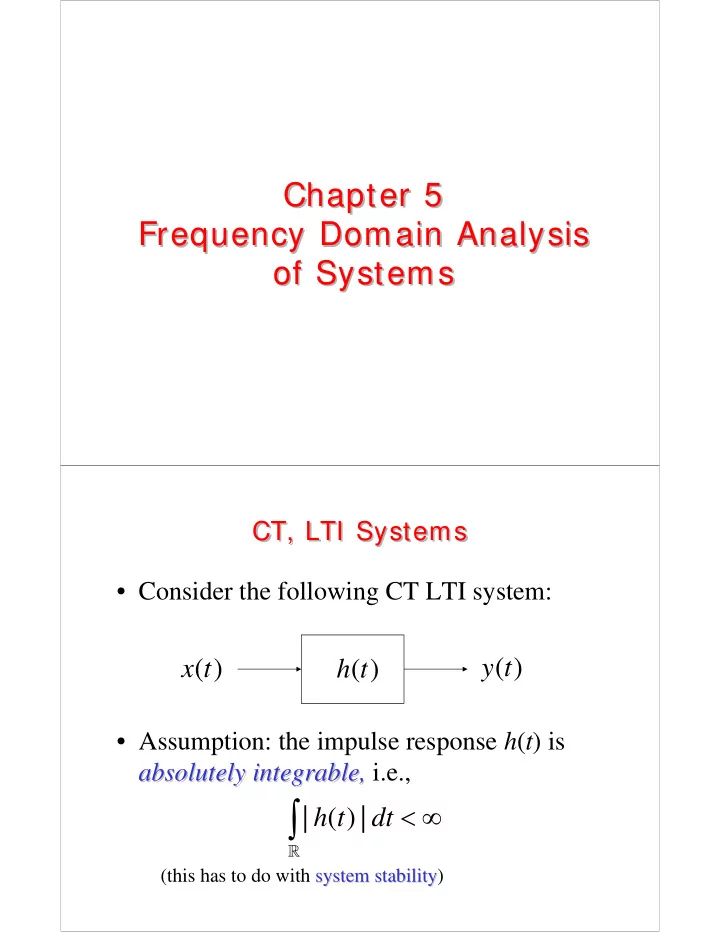
• Consider the following CT LTI system:
• Assumption: the impulse response h(t) is

absolutely absolutely integrable integrable, , i.e., CT, LTI Systems CT, LTI Systems

( ) y t ( ) x t ( ) h t | ( ) | h t dt < ∞

∫

• (this has to do with system stability

system stability)

• What’s the response y(t) of this system to

the input signal

• We start by looking for the response yc(t) of

the same system to Response of a CT, LTI System to a Sinusoidal Input Response of a CT, LTI System to a Sinusoidal Input

( ) cos( ), ? x t t t ω θ = + ∈ ( )

j t c

x t e t

ω

= ∈

• The output is obtained through convolution

as Response of a CT, LTI System to a Complex Exponential Input Response of a CT, LTI System to a Complex Exponential Input

• (

) ( )

( ) ( ) ( ) ( ) ( ) ( ) ( ) ( ) ( )

c

c c c j t j t j x t j c

y t h t x t h x t d h e d e h e d x t h e d

ω τ ω ω τ ω τ

τ τ τ τ τ τ τ τ τ

− − −

= ∗ = − = = = = = =

∫ ∫ ∫ ∫

• By defining

it is

• Therefore, the response of the LTI system to a

complex exponential is another complex exponential with the same frequency The Frequency Response of a CT, LTI System The Frequency Response of a CT, LTI System

( ) ( )

j

H h e d

ωτ

ω τ τ

−

= ∫

• ( )

( ) ( ) ( ) ,

c c j t

y t H x t H e t

ω

ω ω = = = ∈

is the frequency response of the CT, LTI system = Fourier transform of h(t)

( ) H ω

ω

• Since is in general a complex

quantity, we can write Analyzing the Output Signal yc(t) Analyzing the Output Signal yc(t)

arg ( ) ( arg ( ))

( ) ( ) | ( ) | | ( ) |

j t c j H j t j t H

y t H e H e e H e

ω ω ω ω ω

ω ω ω

+

= = = = =

• (

) H ω

• utput signal’s

magnitude

• utput signal’s

phase

• With Euler’s formulas we can express x(t)

as

Using the previous result, the response is

Response of a CT, LTI System to a Sinusoidal Input Response of a CT, LTI System to a Sinusoidal Input

( ) ( ) 1 2 1 1 2 2

( ) cos( ) ( )

j t j t j t j t j j

x t t e e e e e e

ω θ ω θ ω ω θ θ

ω θ

+ − + − −

= + = + = +

1 1 2 2

( ) ( ) ( )

j t j t j j

y t e H e e H e

ω ω θ θ

ω ω

− −

= + −

Response of a CT, LTI System to a Sinusoidal Input – Cont’d Response of a CT, LTI System to a Sinusoidal Input – Cont’d

• If h(t) is real, then

and

• Thus we can write y(t) as

*

( ) ( ) H H ω ω − =

arg ( ) arg ( )

( ) | ( ) | ( ) | ( ) |

j H j H

H H e H H e

ω ω

ω ω ω ω

−

= − =

( arg ( )) ( arg ( ))

1 1 ( ) | ( ) | | ( ) | 2 2 | ( ) | cos( arg ( ))

j t H j t H

y t H e H e H t H

ω θ ω ω θ ω

ω ω ω ω θ ω

+ + − + +

= + = + +

• Thus, the response to

is which is also a sinusoid with the same frequency but with the amplitude amplitude scaled by scaled by the factor the factor and with the phase shifted by amount Response of a CT, LTI System to a Sinusoidal Input – Cont’d Response of a CT, LTI System to a Sinusoidal Input – Cont’d

( ) cos( ) x t A t ω θ = +

( )

( ) cos | arg ( ) ( ) | y t A t H H θ ω ω ω = + + ω | ( ) | H ω arg ( ) H ω

• Suppose that the frequency response of a

CT, LTI system is defined by the following specs: Example: Response of a CT, LTI System to Sinusoidal Inputs Example: Response of a CT, LTI System to Sinusoidal Inputs

1.5, 20, | ( ) | 0, 20, H ω ω ω ≤ ≤ ⎧ = ⎨ > ⎩ arg ( ) 60 , H ω ω = − ∀

• |

( ) | H ω arg ( ) H ω ω ω

20 1.5 60 −

• If the input to the system is
• Then the output is

Example: Response of a CT, LTI System to Sinusoidal Inputs – Cont’d Example: Response of a CT, LTI System to Sinusoidal Inputs – Cont’d

( ) 2cos(10 90 ) 5cos(25 120 ) x t t t = + + +

• |

(10) | | (2 ( ) 2 cos(10 90 ) 5 cos(25 120 arg (10) arg ) 3cos 5) | (10 30 ) (25) H H y t t t t H H = + + + + + + = = +

• Consider the RC circuit shown in figure

Example: Frequency Analysis of an RC Circuit Example: Frequency Analysis of an RC Circuit

• From EEE2032F, we know that:
• 1. The complex impedance

complex impedance of the capacitor is equal to

• 2. If the input voltage is , then the
• utput signal is given by

Example: Frequency Analysis of an RC Circuit – Cont’d Example: Frequency Analysis of an RC Circuit – Cont’d

1/ j C ω

( )

j t c

x t e ω =

1/ 1/ ( ) 1/ 1/

j t j t c

j C RC y t e e R j C j RC

ω ω

ω ω ω = = + +

• Setting , it is

whence we can write where Example: Frequency Analysis of an RC Circuit – Cont’d Example: Frequency Analysis of an RC Circuit – Cont’d

ω ω = 1/ ( ) 1/

j t c

RC y t e j RC

ω

ω = + ( )

j t c

x t e ω =

and and

( ) ( ) ( )

c c

y t H x t ω = 1/ ( ) 1/ RC H j RC ω ω = +

Example: Frequency Analysis of an RC Circuit – Cont’d Example: Frequency Analysis of an RC Circuit – Cont’d

2 2

1/ | ( ) | (1/ ) RC H RC ω ω = +

( )

arg ( ) arctan H RC ω ω = −

1/ 1000 RC =

• The knowledge of the frequency response

allows us to compute the response y(t) of the system to any sinusoidal input signal since Example: Frequency Analysis of an RC Circuit – Cont’d Example: Frequency Analysis of an RC Circuit – Cont’d

( ) H ω ( ) cos( ) x t A t ω θ = +

( )

( ) cos | arg ( ) ( ) | y t A t H H θ ω ω ω = + +

• Suppose that and that
• Then, the output signal is

Example: Frequency Analysis of an RC Circuit – Cont’d Example: Frequency Analysis of an RC Circuit – Cont’d

( ) cos(100 ) cos(3000 ) x t t t = + 1/ 1000 RC =

arg (100) arg (3000 ( ) cos(100 ) cos(3000 ) 0.9950cos(10 | (100) | | (30 5.71 ) 0.3162cos(3 00) | 000 7 ) 1.56 ) y t t t t t H H H H = + + + + = = − + −

• Example: Frequency Analysis of an

RC Circuit – Cont’d Example: Frequency Analysis of an RC Circuit – Cont’d

( ) x t ( ) y t

• Suppose now that

( ) cos(100 ) cos(50,000 ) x t t t = +

Example: Frequency Analysis of an RC Circuit – Cont’d Example: Frequency Analysis of an RC Circuit – Cont’d

• Then, the output signal is

arg (100) arg (50,000) ( ) cos(100 ) cos(50,000 ) 0.9950cos(10 | (100) | | (50,000) 5.71 ) 0.0200cos(50,000 88.85 | ) y t t t t t H H H H = + + + + = = − + −

• Example: Frequency Analysis of an

RC Circuit – Cont’d Example: Frequency Analysis of an RC Circuit – Cont’d

( ) x t ( ) y t

The RC circuit behaves as a lowpass lowpass filter filter, by letting low- frequency sinusoidal signals pass with little attenuation and by significantly attenuating high-frequency sinusoidal signals

• Suppose that the input to the CT, LTI

system is a periodic signal periodic signal x(t) having period T

• This signal can be represented through its

Fourier series Fourier series as Response of a CT, LTI System to Periodic Inputs Response of a CT, LTI System to Periodic Inputs

( ) ,

jk t x k k

x t c e t

ω ∞ =−∞

= ∈

∑

• 1

( ) ,

t T jk t x k t

c x t e dt k T

ω + −

= ∈

∫

• where
• By exploiting the previous results and the

linearity of the system, the output of the system is Response of a CT, LTI System to Periodic Inputs – Cont’d Response of a CT, LTI System to Periodic Inputs – Cont’d

( ar arg ( g( ) ) | ) | ( arg( ) )

| ( ) ( ) | ( ) | | | | ,

x k y k y k

jk t x k k j k t c x k k c j k t c jk t y y k k k k k H

y t H k c e c e c e t k c e H

ω ω ω ω ω

ω ω

∞ =−∞ ∞ + + =−∞ ∞ ∞ + =−∞ =−∞

= = = = = ∈

∑ ∑ ∑ ∑

• arg

y k

c

Example: Response of an RC Circuit to a Rectangular Pulse Train Example: Response of an RC Circuit to a Rectangular Pulse Train

• Consider the RC circuit

with input ( )

rect( 2 )

n

x t t n

∈

= −

∑

• We have found its Fourier series to be

with Example: Response of an RC Circuit to a Rectangular Pulse Train – Cont’d Example: Response of an RC Circuit to a Rectangular Pulse Train – Cont’d

( ) ,

x jk t k k

x t c e t

π ∈

= ∈

∑

• 1 sinc

2 2

x k

k c ⎛ ⎞ = ⎜ ⎟ ⎝ ⎠

( ) rect( 2 )

n

x t t n

∈

= −

∑

• Magnitude spectrum of input signal x(t)

Example: Response of an RC Circuit to a Rectangular Pulse Train – Cont’d Example: Response of an RC Circuit to a Rectangular Pulse Train – Cont’d

| |

x k

c

• The frequency response of the RC circuit

was found to be

• Thus, the Fourier series of the output signal

is given by Example: Response of an RC Circuit to a Rectangular Pulse Train – Cont’d Example: Response of an RC Circuit to a Rectangular Pulse Train – Cont’d

1/ ( ) 1/ RC H j RC ω ω = + ( ) ( )

jk t jk t x y k k k k

y t H k c e c e

ω ω

ω

∞ ∞ =−∞ =−∞

= =

∑ ∑

Example: Response of an RC Circuit to a Rectangular Pulse Train – Cont’d Example: Response of an RC Circuit to a Rectangular Pulse Train – Cont’d

| ( ) | ( ) H dB ω

ω

1/ 1 RC = 1/ 10 RC = 1/ 100 RC =

filter more selective

Example: Response of an RC Circuit to a Rectangular Pulse Train – Cont’d Example: Response of an RC Circuit to a Rectangular Pulse Train – Cont’d

| |

y k

c

1/ 1 RC =

| |

y k

c | |

y k

c

1/ 100 RC = 1/ 10 RC =

filter more selective

Example: Response of an RC Circuit to a Rectangular Pulse Train – Cont’d Example: Response of an RC Circuit to a Rectangular Pulse Train – Cont’d

( ) y t ( ) y t ( ) y t

1/ 1 RC = 1/ 10 RC = 1/ 100 RC =

filter more selective

• Consider the following CT, LTI system
• Its I/O relation is given by

which, in the frequency domain, becomes Response of a CT, LTI System to Aperiodic Inputs Response of a CT, LTI System to Aperiodic Inputs

( ) y t ( ) x t ( ) h t ( ) ( ) ( ) y t h t x t = ∗ ( ) ( ) ( ) Y H X ω ω ω =

• From , the magnitude

magnitude spectrum spectrum of the output signal y(t) is given by and its phase spectrum phase spectrum is given by Response of a CT, LTI System to Aperiodic Inputs – Cont’d Response of a CT, LTI System to Aperiodic Inputs – Cont’d

( ) ( ) ( ) Y H X ω ω ω = arg ( ) arg arg ( ( ) ) H Y X ω ω ω = + | ( | ( ) | | | ( ) | ) H Y X ω ω ω =

Example: Response of an RC Circuit to a Rectangular Pulse Example: Response of an RC Circuit to a Rectangular Pulse

• Consider the RC circuit

with input

( ) rect( ) x t t =

• The Fourier transform of x(t) is

Example: Response of an RC Circuit to a Rectangular Pulse – Cont’d Example: Response of an RC Circuit to a Rectangular Pulse – Cont’d

( ) rect( ) x t t =

( ) sinc 2 X ω ω π ⎛ ⎞ = ⎜ ⎟ ⎝ ⎠

Example: Response of an RC Circuit to a Rectangular Pulse – Cont’d Example: Response of an RC Circuit to a Rectangular Pulse – Cont’d

| ( ) | X ω arg ( ) X ω

Example: Response of an RC Circuit to a Rectangular Pulse – Cont’d Example: Response of an RC Circuit to a Rectangular Pulse – Cont’d

| ( ) | Y ω arg ( ) Y ω

1/ 1 RC =

Example: Response of an RC Circuit to a Rectangular Pulse – Cont’d Example: Response of an RC Circuit to a Rectangular Pulse – Cont’d

1/ 10 RC =

| ( ) | Y ω arg ( ) Y ω

• The response of the system in the time

domain can be found by computing the convolution where Example: Response of an RC Circuit to a Rectangular Pulse – Cont’d Example: Response of an RC Circuit to a Rectangular Pulse – Cont’d

(1/ )

( ) (1/ ) ( )

RC t

h t RC e u t

−

= ( ) rect( ) x t t = ( ) ( ) ( ) y t h t x t = ∗

Example: Response of an RC Circuit to a Rectangular Pulse – Cont’d Example: Response of an RC Circuit to a Rectangular Pulse – Cont’d

1/ 1 RC = 1/ 10 RC =

( ) y t ( ) y t

filter more selective

Example: Attenuation of High- Frequency Components Example: Attenuation of High- Frequency Components

( ) Y ω ( ) H ω ( ) X ω

=

×

Example: Attenuation of High- Frequency Components Example: Attenuation of High- Frequency Components

( ) y t ( ) x t

• The response of a CT, LTI system with

frequency response to a sinusoidal signal

• Filtering

Filtering: if or then or Filtering Signals Filtering Signals

( ) cos( ) x t A t ω θ = +

( )

( ) cos | arg ( ) ( ) | y t A t H H θ ω ω ω = + + ( ) H ω | ( ) | 0 H ω = | ( ) | 0 H ω ≈ ( ) y t = ( ) 0, y t t ≈ ∀ ∈

is is Four Basic Types of Filters Four Basic Types of Filters

lowpass lowpass

| ( ) | H ω | ( ) | H ω | ( ) | H ω | ( ) | H ω

bandstop bandstop bandpass bandpass highpass highpass

passband passband cutoff frequency cutoff frequency stopband stopband stopband stopband

• Filters are usually designed based on

specifications on the magnitude response

• The phase response has to be taken

into account too in order to prevent signal distortion as the signal goes through the system

• If the filter has linear phase

linear phase in its passband(s), then there is no distortion no distortion Phase Function Phase Function

| ( ) | H ω arg ( ) H ω

• Consider the ideal sampler:
• It is convenient to express the sampled signal

as where Ideal Sampling Ideal Sampling

( ) x t [ ] ( ) ( )

t nT

x n x t x nT

=

= =

. .

T n∈ ( ) x nT ( ) ( ) x t p t ( ) ( )

n

p t t nT δ

∈

= −

∑

• t ∈

• Thus, the sampled waveform is
• is an impulse train whose weights

(areas) are the sample values of the

• riginal signal x(t)

Ideal Sampling – Cont’d Ideal Sampling – Cont’d

( ) ( ) ( ) ( ) ( ) ( )

n n

x t p t x t t nT x nT t nT δ δ

∈ ∈

= − = −

∑ ∑

• ( ) ( )

x t p t ( ) ( ) x t p t ( ) x nT

• Since p(t) is periodic with period T, it can

be represented by its Fourier series Fourier series Ideal Sampling – Cont’d Ideal Sampling – Cont’d

2 ( ) ,

s

jk t k s k

p t c e T

ω

π ω

∈

= =

∑

• sampling

sampling frequency frequency ( (rad rad/sec) /sec)

/ 2 / 2 / 2 / 2

1 ( ) , 1 1 ( )

s s

T jk t k T T jk t T

c p t e dt k T t e dt T T

ω ω

δ

− − − −

= ∈ = =

∫ ∫

• where

where

• Therefore

and whose Fourier transform is Ideal Sampling – Cont’d Ideal Sampling – Cont’d

1 ( )

s

jk t k

p t e T

ω ∈

= ∑

• 1

1 ( ) ( ) ( ) ( ) ( )

s s

jk t jk t s k k

x t x t p t x t e x t e T T

ω ω ∈ ∈

= = =

∑ ∑

• 1

( ) ( )

s s k

X X k T ω ω ω

∈

= −

∑

• Ideal Sampling – Cont’d

Ideal Sampling – Cont’d

1 ( ) ( )

s s k

X X k T ω ω ω

∈

= −

∑

• ( )

X ω

• Suppose that the signal x(t) is bandlimited

with bandwidth B, i.e.,

• Then, if the replicas of in

do not overlap and can be recovered by applying an ideal lowpass filter to (interpolation filter interpolation filter) Signal Reconstruction Signal Reconstruction

| ( ) | 0, for | | X B ω ω = > 2 ,

s

B ω ≥ ( ) X ω 1 ( ) ( )

s s k

X X k T ω ω ω

∈

= −

∑

• ( )

X ω ( )

s

X ω

Interpolation Filter for Signal Reconstruction Interpolation Filter for Signal Reconstruction

, [ , ] ( ) 0, [ , ] T B B H B B ω ω ω ∈ − ⎧ = ⎨ ∉ − ⎩

• The impulse response h(t) of the interpolation

filter is and the output y(t) of the interpolation filter is given by Interpolation Formula Interpolation Formula

B ( ) sinc BT h t t π π ⎛ ⎞ = ⎜ ⎟ ⎝ ⎠ ( ) ( ) ( )

s

y t h t x t = ∗

• But

whence

• Moreover,

Interpolation Formula – Cont’d Interpolation Formula – Cont’d

( ) ( ) ( ) ( ) ( )

s n

x t x t p t x nT t nT δ

∈

= = −

∑

• ( )

( ) ( ) ( ) ( ) ( )sinc ( )

s n n

y t h t x t x nT h t nT BT B x nT t nT π π

∈ ∈

= ∗ = − = ⎛ ⎞ = − ⎜ ⎟ ⎝ ⎠

∑ ∑

• ( )

( ) y t x t =

• A CT bandlimited signal x(t) with frequencies

no higher than B can be reconstructed from its samples if the samples are taken at a rate

• The reconstruction of x(t) from its samples

is provided by the interpolation formula Shannon’s Sampling Theorem Shannon’s Sampling Theorem

[ ] ( ) x n x nT = 2 / 2

s

T B ω π = ≥ si ( n ) c ) ( ) (

n

B x T B t T x t nT n π π

∈

⎛ ⎞ = − ⎜ ⎟ ⎝ ⎠

∑

• (

[ ) ] x x n nT =

• The minimum sampling rate

is called the Nyquist rate

• Question: Why do CD’s adopt a sampling

rate of 44.1 kHz?

• Answer: Since the highest frequency

perceived by humans is about 20 kHz, 44.1 kHz is slightly more than twice this upper bound Nyquist Rate Nyquist Rate

2 / 2

s

T B ω π = =

Aliasing Aliasing

1 ( ) ( )

s s k

X X k T ω ω ω

∈

= −

∑

• ( )

X ω

• Because of aliasing, it is not possible to

reconstruct x(t) exactly by lowpass filtering the sampled signal

• Aliasing results in a distorted version of the
• riginal signal x(t)
• It can be eliminated (theoretically) by

lowpass filtering x(t) before sampling it so that for Aliasing –Cont’d Aliasing –Cont’d

( ) ( ) ( )

s

x t x t p t = | ( ) | 0 X ω = | | B ω ≥