dt < | ( ) | h t (this has to do with system stability - PDF document

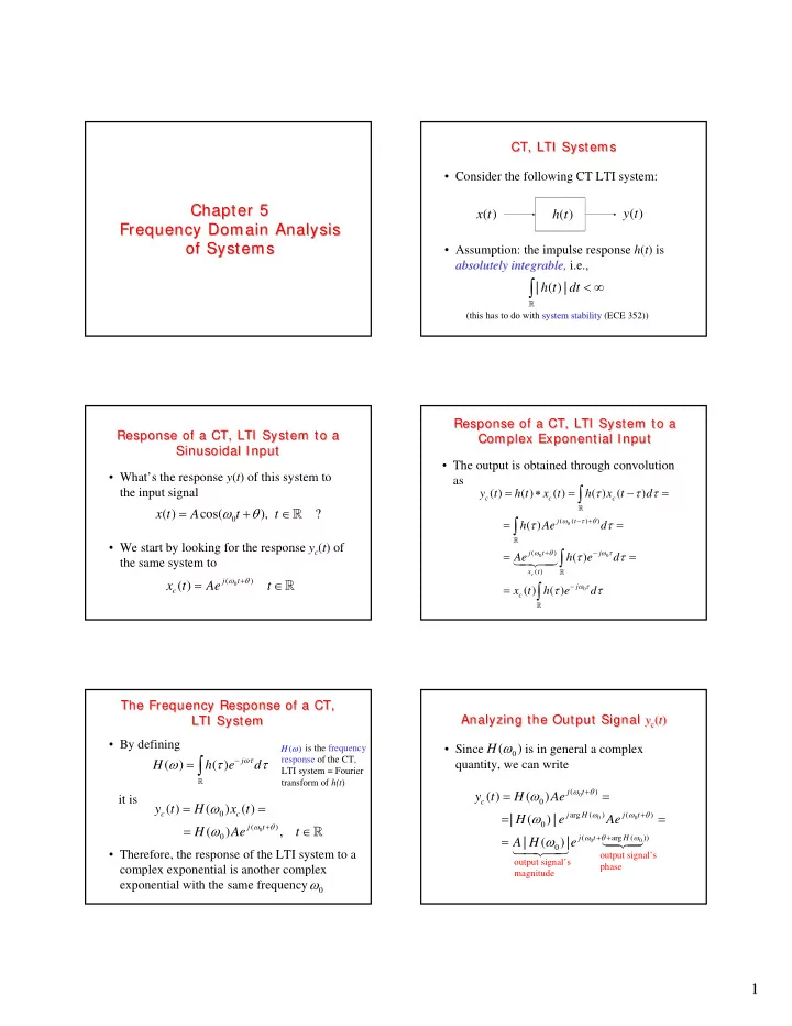
CT, LTI Systems CT, LTI Systems • Consider the following CT LTI system: Chapter 5 Chapter 5 ( ) ( ) ( ) x t h t y t Frequency Domain Analysis Frequency Domain Analysis of Systems of Systems • Assumption: the impulse response h ( t ) is absolutely integrable integrable, , i.e., absolutely ∫ dt < ∞ | ( ) | h t � (this has to do with system stability system stability (ECE 352)) Response of a CT, LTI System to a Response of a CT, LTI System to a Response of a CT, LTI System to a Response of a CT, LTI System to a Complex Exponential Input Complex Exponential Input Sinusoidal Input Sinusoidal Input • The output is obtained through convolution • What’s the response y ( t ) of this system to as ∫ = ∗ = τ − τ τ = the input signal ( ) ( ) ( ) ( ) ( ) y t h t x t h x t d c c c = ω + θ ∈ � � x t ( ) A cos( t ), t ? 0 ∫ = τ ω − τ + θ τ = ( ( ) ) j t h ( ) Ae d 0 � • We start by looking for the response y c ( t ) of ω + θ ∫ − ω τ = τ τ = j ( t ) j ( ) Ae h e d � � �� 0 � 0 the same system to ( ) � x t c = ω + θ ∈ � ( ) j t ( ) ∫ x t Ae 0 t − ω τ = τ τ j ( ) ( ) x t h e 0 d c c � The Frequency Response of a CT, The Frequency Response of a CT, Analyzing the Output Signal y c ( t ) LTI System LTI System Analyzing the Output Signal y c ( t ) • By defining H ω H ω ( ) is the frequency • Since is in general a complex ( ) = ∫ 0 − ωτ ω τ τ response of the CT, j ( ) ( ) quantity, we can write H h e d LTI system = Fourier � transform of h(t ) = ω ω + θ = ( ) j t ( ) ( ) y t H Ae 0 it is c 0 = ω = ( ) ( ) ( ) y t H x t ω ω + θ 0 = ω = c c j arg H ( ) j ( t ) | H ( ) | e Ae 0 0 0 = ω ω + θ ∈ � ( ) j t ( ) , H Ae 0 t = � ω ω + + θ ω 0 ( � � arg � � � ( )) j t H | ( ) | A H e 0 0 � �� � 0 • Therefore, the response of the LTI system to a output signal’s output signal’s phase complex exponential is another complex magnitude ω exponential with the same frequency 0 1 1

Response of a CT, LTI System to a Response of a CT, LTI System to a Response of a CT, LTI System to a Response of a CT, LTI System to a Sinusoidal Input Sinusoidal Input Sinusoidal Input – Cont’d Sinusoidal Input – Cont’d • Thus, the response to • With Euler’s formulas we can express = ω + θ = ω + θ ( ) cos( ) x t A t ( ) cos( ) x t A t 0 0 is as ( ) = ω ω + θ + ω ∗ = ℜ = + ( ) | ( ) | cos arg ( ) ( ) ( ( )) 1 ( ( ) ( )) y t A H t H x t x t x t x t 0 0 0 c 2 c c which is also a sinusoid with the same and, by exploiting linearity exploiting linearity, it is ω frequency but with the amplitude amplitude scaled by scaled by 0 = ℜ = + ∗ = 1 H ω y t ( ) ( y t ( )) ( y t ( ) y t ( )) the factor the factor | ( ) | and with the phase shifted c 2 c c 0 H ω ( ) = ω ω + θ + ω by amount arg ( ) | ( ) | cos arg ( ) A H t H 0 0 0 0 Response of a DT, LTI System to a Response of a DT, LTI System to a DT, LTI Systems DT, LTI Systems Complex Exponential Input Complex Exponential Input • Consider the following DT, LTI system: • If the input signal is ω + θ = ∈ � j ( n ) x n [ ] Ae n 0 c [ ] [ ] [ ] x n h n y n • Then the output signal is given by = ω = [ ] ( ) [ ] y n H x n c 0 c • The I/O relation is given by ω + θ = ω ∈ � j ( n ) H ( ) Ae , n 0 0 where = ∗ H ω is the frequency y n [ ] h n [ ] x n [ ] ( ) ∑ ω = − ω ω ∈ � response of the DT, LTI j k ( ) [ ] , H h k e system = DT Fourier ∈ � k transform (DTFT) of h [ n ] Example: Response of a CT, LTI Example: Response of a CT, LTI Response of a DT, LTI System to a Response of a DT, LTI System to a System to Sinusoidal Inputs System to Sinusoidal Inputs Sinusoidal Input Sinusoidal Input • Suppose that the frequency response of a • If the input signal is CT, LTI system is defined by the following = ω + θ ∈ � [ ] cos( ) x n A n n specs: 0 • Then the output signal is given by H ω ≤ ω ≤ | ( ) | ⎧ ( ) 1.5, 0 20, = ω ω + θ + ω 1.5 [ ] | ( ) | cos arg ( ) ω = ⎨ y n A H n H | ( ) | H 0 0 0 ω > ⎩ 0, 20, 0 ω 20 H ω arg ( ) H ω = − � ∀ ω ω arg ( ) 60 , − � 60 2 2

Example: Response of a CT, LTI Example: Response of a CT, LTI Example: Frequency Analysis of an Example: Frequency Analysis of an System to Sinusoidal Inputs – System to Sinusoidal Inputs – RC Circuit RC Circuit Cont’d Cont’d • If the input to the system is • Consider the RC circuit shown in figure = + � + + � ( ) 2cos(10 90 ) 5cos(25 120 ) x t t t • Then the output is = + � + + ( ) 2 | (10) | cos(10 90 arg (10) ) y t H t H + + + = � 5 | (2 5) | cos(25 120 arg (25) ) H t H = + � 3cos (10 30 ) t Example: Frequency Analysis of an Example: Frequency Analysis of an Example: Frequency Analysis of an Example: Frequency Analysis of an RC Circuit – Cont’d RC Circuit – Cont’d RC Circuit – Cont’d RC Circuit – Cont’d = j ω • From ENGR 203, we know that: • Setting , it is s 0 1. The complex impedance complex impedance of the capacitor is 1/ RC ω = = e ω j t = σ + ω j t y t ( ) e ( ) 0 1/ sC s j x t 0 and equal to where and ω + c c 1/ j RC = st x t ( ) e 0 2. If the input voltage is , then the c whence we can write output signal is given by = ω ( ) ( ) ( ) y t H x t 1/ 1/ sC RC c 0 c = = st st y t ( ) e e where + + c 1/ 1/ R sC s RC 1/ RC ω = H ( ) ω + 1/ j RC Example: Frequency Analysis of an Example: Frequency Analysis of an Example: Frequency Analysis of an Example: Frequency Analysis of an RC Circuit – Cont’d RC Circuit – Cont’d RC Circuit – Cont’d RC Circuit – Cont’d 1/ RC ω = | H ( ) | • The knowledge of the frequency response ω + 2 2 (1/ ) RC H ω ( ) allows us to compute the response y ( t ) of the system to any sinusoidal input signal = ω + θ ( ) cos( ) x t A t ( ) 0 ω = − ω arg ( ) arctan H RC since ( ) = ω ω + θ + ω y t ( ) A | H ( ) | cos t arg H ( ) 0 0 0 RC = 1/ 1000 3 3

Example: Frequency Analysis of an Example: Frequency Analysis of an Example: Frequency Analysis of an Example: Frequency Analysis of an RC Circuit – Cont’d RC Circuit – Cont’d RC Circuit – Cont’d RC Circuit – Cont’d ( ) x t RC = • Suppose that and that 1/ 1000 = + x t ( ) cos(100 ) t cos(3000 ) t • Then, the output signal is ( ) y t = + + ( ) | (100) | cos(100 arg (100) ) y t H t H + + = | H (30 00) | cos(3000 t arg H (3000 ) ) = − � + − � 0.9950cos(10 0 t 5.71 ) 0.3162cos(3 000 t 7 1.56 ) Example: Frequency Analysis of an Example: Frequency Analysis of an Example: Frequency Analysis of an Example: Frequency Analysis of an RC Circuit – Cont’d RC Circuit – Cont’d RC Circuit – Cont’d RC Circuit – Cont’d x t ( ) y t ( ) • Suppose now that = + ( ) cos(100 ) cos(50,000 ) x t t t •Then, the output signal is = + + y t ( ) | H (100) | cos(100 t arg H (100) ) + + = | (50,000) | cos(50,000 arg (50,000) ) H t H = − � + − � 0.9950cos(10 0 5.71 ) 0.0200cos(50,000 88.85 ) t t The RC circuit behaves as a lowpass lowpass filter filter, by letting low- frequency sinusoidal signals pass with little attenuation and by significantly attenuating high-frequency sinusoidal signals Response of a CT, LTI System to Response of a CT, LTI System to Response of a CT, LTI System to Response of a CT, LTI System to Periodic Inputs Periodic Inputs – Cont’d Periodic Inputs Periodic Inputs – Cont’d • By exploiting the previous results and the • Suppose that the input to the CT, LTI linearity of the system, the output of the system is a periodic signal periodic signal x ( t ) having system is period T ∞ ∑ ω = ω x jk t • This signal can be represented through its ( ) ( ) y t H k c e 0 0 k =−∞ Fourier series as Fourier series k ∞ ∞ ∑ ω + �� + �� � ω ∑ = ω x = x j k ( t ar g( c ) arg H ( k ) ) ω | ( ) | | | = ∈ H k c e x jk t � 0 k 0 ( ) , x t c e t �� � ��� � 0 0 k y k =−∞ arg c k =−∞ k k y | c | k + where t T ∞ ∞ 1 0 ∫ ∑ ∑ − ω = ∈ ω + y ω x jk t � = ( arg( ) ) = ∈ y j k t c y jk t � c x t e ( ) dt , k | | , 0 c e 0 c e 0 t k k k k T =−∞ =−∞ k k t 0 4 4