
SLIDE 1
Deep Neural Networks and Mixed Integer Linear Optimization
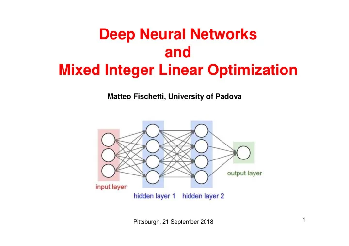
Matteo Fischetti, University of Padova
Pittsburgh, 21 September 2018 1
Deep Neural Networks and Mixed Integer Linear Optimization Matteo - - PowerPoint PPT Presentation
Deep Neural Networks and Mixed Integer Linear Optimization Matteo Fischetti, University of Padova 1 Pittsburgh, 21 September 2018 Machine Learning Example (MIPpers only!): Continuous 0-1 Knapack Problem with a fixed n. of items
Pittsburgh, 21 September 2018 1
Pittsburgh, 21 September 2018 2
Pittsburgh, 21 September 2018 3
Pittsburgh, 21 September 2018 4
Pittsburgh, 21 September 2018 5
Pittsburgh, 21 September 2018 6
– define an optimization problem where the parameters are the unknowns – (huge) training set of points x for which we know the “true” value f*(x) –
terms) to be minimized on the training set (but … not too much!) – validation set: can be used to select “hyperparameters” not directly handled by the optimizer (it plays a crucial role indeed…) – test set: points not seen during training, used to evaluate the actual accuracy of the DNN on (future) unseen data.
Pittsburgh, 21 September 2018 7
Pittsburgh, 21 September 2018 8
Pittsburgh, 21 September 2018 9
Pittsburgh, 21 September 2018 10
Pittsburgh, 21 September 2018 11
Pittsburgh, 21 September 2018 12
Pittsburgh, 21 September 2018 13
Pittsburgh, 21 September 2018 14
regions of deep neural networks. CoRR arXiv:1711.02114. Pittsburgh, 21 September 2018 15
Pittsburgh, 21 September 2018 16
Pittsburgh, 21 September 2018 17
Pittsburgh, 21 September 2018 18
Pittsburgh, 21 September 2018 19
On handling indicator constraints in mixed integer programming. Computational Optimization and Applications, (65):545–566, 2016.
Pittsburgh, 21 September 2018 20
Pittsburgh, 21 September 2018 21
Pittsburgh, 21 September 2018 22
Pittsburgh, 21 September 2018 23
Programs: A Feasibility Study", 2017, arXiv preprint arXiv:1712.06174 (accepted in CPAIOR 2018) .
Pittsburgh, 21 September 2018 24