Drag Prediction Using Automatic Hexahedra Grid Generation Method - PowerPoint PPT Presentation

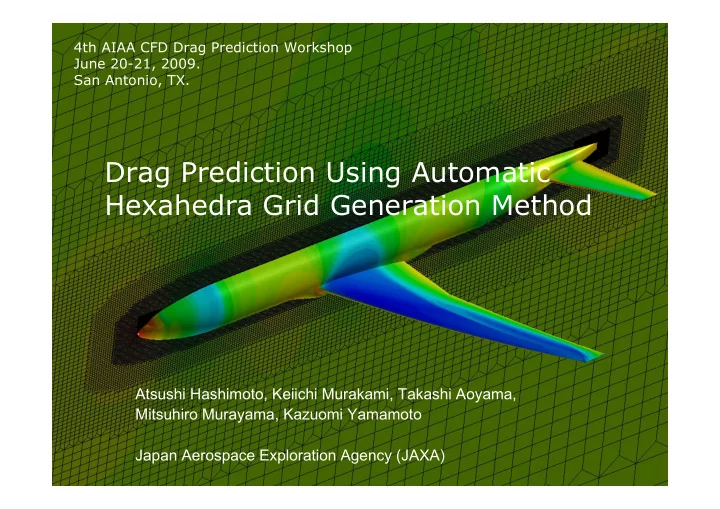
4th AIAA CFD Drag Prediction Workshop June 20-21, 2009. San Antonio, TX. Drag Prediction Using Automatic Hexahedra Grid Generation Method Atsushi Hashimoto, Keiichi Murakami, Takashi Aoyama, Mitsuhiro Murayama, Kazuomi Yamamoto Japan Aerospace Exploration Agency (JAXA) 1

Objective The objective of this study is evaluation of an automatic hexahedra grid generator, HexaGrid. Contents � Features of HexaGrid -Grid generated by HexaGrid � Flow solver (TAS) � Results - Comparison with JAXA’s other results. (MEGG3D+TAS, Gridgen+UPACS) 2

Features of HexaGrid HexaGrid : Automatic grid generator based on hexahedral grid • Unstructured mesh based on Cartesian mesh • Handles complex geometry • Automatic operation (very few control parameters) • Predominantly hexahedral element • Input multi-component geometry in STL format • Run on ordinary PC and JSS (JAXA Supercomputer System). 3

Input parameters Automatic operation using very few control parameters � Domain (max and min of x, y, z) Max and min cell size on the surface � � Layer parameter (thickness of first layer, expansion factor) 4

Mesh Refinement Control • Start with one big element (= computational domain) • Cartesian grid is generated by means of successive local refinement • Each refinement divides a cell isotropically into eight child cells • Refine the element using 3 criteria • Each criterion has a target element size (user-defined) (1) Region refined by solid surface (user defines max cell size) (3) Refinement box (user defines box position and cell size) (2) Region refined by solid surface with large curvature (user defines min cell size) 5 We do not use the refinement box for simplicity in this study .

Prismatic grid generation Thickness of first layer and expansion factor are given by the input parameters Grid surface snapped to solid surface Prismatic grid generation 6 Grid smoothing

Feature capturing Feature capturing Without feature capturing STL data With feature capturing Grid surface 7

Setting of gridding parameters Upper surface of main wing Setting parameter Coarse Medium Fine Max cell size on solid surface 5 in 5 in 5 in Min cell size on solid surface 5 in 1.25 in (=5/2 2 ) 0.625 in (=5/2 3 ) Expansion ratio of prism layers 1.25 1.25 1.25 Thickness of first prism layer 9.85E-4 in 9.85E-4 in 9.85E-4 in Cubic domain size 100 C ref 100 C ref 100 C ref Reference Chord length = 275.80 in Gridding Guidelines 8

Setting of gridding parameters Upper surface of main wing Setting parameter Coarse Medium Fine Max cell size on solid surface 5 in 5 in 5 in Min cell size on solid surface 5 in 1.25 in (=5/2 2 ) 0.625 in (=5/2 3 ) Expansion ratio of prism layers 1.25 1.25 1.25 Thickness of first prism layer 9.85E-4 in 9.85E-4 in 9.85E-4 in 0.1% of local chord at LE, TE � 0.11-0.47in for the main wing (Gridding Guidelines) Cubic domain size 100 C ref 100 C ref 100 C ref � 10-50 times larger grid size (Coarse grid) Reference Chord length = 275.80 in 3-10 times larger grid size (Medium grid) Gridding Guidelines 1.5-6 times larger grid size (Fine grid) 9

Grids generated with HexaGrid Body/main wing juncture Coarse Medium Fine +2 +3 Coarse Medium Fine � Feature line is Number of refinement process 13 15 16 clearly captured Number of prism layers 35 29 26 Node count 3,213,783 11,055,602 36,601,899 Cell count 3,644,942 12,654,764 41,630,191 Boundary node count 105,686 295,394 757,593 Boundary face count 106,272 297,697 762,131 Prismatic cell count 1,932,525 7,145,542 17,752,826 3.5M (Coarse), 10M (medium), 35M (fine) are required by the guideline. 10

Grids generated with HexaGrid Wing tip of main wing Coarse Medium Fine +2 +3 Coarse Medium Fine Number of refinement process 13 15 16 Number of prism layers 35 29 26 Node count 3,213,783 11,055,602 36,601,899 Cell count 3,644,942 12,654,764 41,630,191 Boundary node count 105,686 295,394 757,593 Boundary face count 106,272 297,697 762,131 Prismatic cell count 1,932,525 7,145,542 17,752,826 3.5M (Coarse), 10M (medium), 35M (fine) are required by the guideline. 11

Grids generated with HexaGrid Tail wing Coarse Medium Fine +2 +3 Coarse Medium Fine Number of refinement process 13 15 16 Number of prism layers 35 29 26 Node count 3,213,783 11,055,602 36,601,899 Cell count 3,644,942 12,654,764 41,630,191 Boundary node count 105,686 295,394 757,593 Boundary face count 106,272 297,697 762,131 Prismatic cell count 1,932,525 7,145,542 17,752,826 3.5M (Coarse), 10M (medium), 35M (fine) are required by the guideline. 12

Grids generated with HexaGrid Cross-section of main wing at eta=0.50 Coarse Medium Fine +2 +3 Coarse Medium Fine Number of refinement process 13 15 16 Number of prism layers 35 29 26 Node count 3,213,783 11,055,602 36,601,899 Cell count 3,644,942 12,654,764 41,630,191 Boundary node count 105,686 295,394 757,593 Boundary face count 106,272 297,697 762,131 Prismatic cell count 1,932,525 7,145,542 17,752,826 3.5M (Coarse), 10M (medium), 35M (fine) are required by the guideline. 13

Grids generated with HexaGrid Trailing edge of main wing at eta=0.50 Coarse Medium Fine +2 +3 Coarse Medium Fine � 5-6 nodes are Number of refinement process 13 15 16 located across the TE Number of prism layers 35 29 26 base. Node count 3,213,783 11,055,602 36,601,899 � The total thickness Cell count 3,644,942 12,654,764 41,630,191 of prism layer is Boundary node count 105,686 295,394 757,593 decreasing. Boundary face count 106,272 297,697 762,131 Prismatic cell count 1,932,525 7,145,542 17,752,826 3.5M (Coarse), 10M (medium), 35M (fine) are required by the guideline. 14

Flow Solver Configuration TAS-code ( T ohoku University A erodynamic S imulation code) � Mesh: Unstructured grid � Discretization: Cell vertex, finite volume method � Flux: HLLEW (Harten-Lax-van Leer-Einfeldt-Wada) � Accuracy: Second order by a linear reconstruction with Venkatakrishnan’s limiter and U-MUSCL � Time integration: LU-SGS � Turbulence model: Spalart-Allmaras (SA) As for the SA model, the trip term and the ft2 function are not included. A modified production term is used. 15

Results Cp contours (M=0.85, CL=0.50, Medium Grid) 16

1.1 Grid convergence study M=0.85, CL=0.50 Coarse, medium, fine grids 0.0295 0.53 HexaGrid+TAS 0.52 0.0290 0.51 0.50 0.0285 0.49 CD 0.48 Coarse CL Medium 0.47 0.0280 Fine 0.46 0.45 0.0275 0.44 0.43 0.42 0.0270 0.022 0.024 0.026 0.028 0.03 0.032 0.E+00 1.E-05 2.E-05 3.E-05 4.E-05 5.E-05 CD 1/(Gridsize)^(2/3) 17

1.2 Downwash study 0.7 0.7 0.6 0.6 0.5 0.5 iH=-2 0.4 0.4 iH=0 CL CL iH=2 iH=-2 0.3 0.3 No tail iH=0 iH=2 0.2 0.2 No tail 0.1 0.1 0 0 0.015 0.025 0.035 0.045 0.055 0 1 2 3 4 5 AoA CD 0.7 0.7 iH=0 0.6 0.6 iH=-2 0.5 iH=2 0.5 No tail iH=-2 0.4 0.4 iH=0 CL CL iH=2 0.3 0.3 No tail 0.2 0.2 0.1 0.1 0 0 0.015 0.02 0.025 0.03 0.035 -0.4 -0.3 -0.2 -0.1 0 0.1 0.2 0.3 18 2 / π AR =C D -C L Idealized CD CM

Trim Drag TRIMMED DRAG POLAR => Interpolate iH at fixed CL to calculate CM_TOT = 0. 0.7 0.6 0.5 iH=-2 iH=0 0.4 CL iH=2 0.3 No tail Trimed 0.2 0.1 0 0.015 0.025 0.035 0.045 0.055 19 CD

2 Mach sweep study CD at CL=0.4, 0.45, and 0.5 for M=0.7-0.87 0.034 CL=0.4 0.032 CL=0.45 0.03 CL=0.5 0.028 CD 0.026 0.024 0.022 0.02 0.7 0.75 0.8 0.85 0.9 Mach number 20

Comparison with other results Hexa unstructured grid HexaGrid + TAS Tetra unstructured grid MEGG3D + TAS Multi-block structured grid Gridgen + UPACS 21

Grid convergence study 0.0295 HexaGrid+TAS Grid convergence study of iH=0 model MEGG3D+TAS 0.0290 UPACS at CL=0.500, M=0.85 0.0285 � Large sensitivity of grid size CD 0.0280 � HexaGrid+TAS results are between 0.0275 MEGG3D+TAS and UPACS. (The results of HexaGrid are comparable CD_total 0.0270 to the manual methods.) 0.0265 0.E+00 1.E-05 2.E-05 3.E-05 4.E-05 5.E-05 1/(Gridsize)^(2/3) 0.0175 0.0127 CD_pressure CD_skin-friction HexaGrid+TAS 0.0170 0.0126 MEGG3D+TAS UPACS 0.0165 0.0125 CD_pressure CD_friction 0.0160 0.0124 0.0155 0.0123 0.0150 0.0122 HexaGrid+TAS MEGG3D+TAS 0.0145 0.0121 UPACS 0.0140 0.012 0.E+00 1.E-05 2.E-05 3.E-05 4.E-05 5.E-05 0.E+00 1.E-05 2.E-05 3.E-05 4.E-05 5.E-05 22 1/(Gridsize)^(2/3) 1/(Gridsize)^(2/3)

Cp distribution (Medium, iH=0, CL=0.5) -1.2 -1.2 -1 -1 HexaGrid+TAS HexaGrid+TAS MEGG3D+TAS MEGG3D+TAS -0.8 -0.8 UPACS UPACS -0.6 -0.6 η=0.30 Eta=0.30 η=0.20 Eta=0.2 -0.4 -0.4 Cp -0.2 Cp -0.2 0 0.2 0.4 0.6 0.8 1 0 0.2 0.4 0.6 0.8 1 Eta=0.5 η=0.50 0 0 0.2 0.2 Eta=0.2 Eta=0.5 0.4 0.4 η=0.95 Eta=0.95 0.6 0.6 0.8 0.8 x/c x/c � HexaGrid results agree well -0.8 -0.8 with the other results. HexaGrid+TAS -0.6 -0.6 MEGG3D+TAS HexaGrid+TAS UPACS MEGG3D+TAS -0.4 -0.4 UPACS � The shock wave in the -0.2 -0.2 middle of wing is well 0 0.2 0.4 0.6 0.8 1 0 0.2 0.4 0.6 0.8 1 Cp 0 0 captured with HexaGrid. 0.2 0.2 Eta=0.95 0.4 0.4 Eta=0.3 (tail) � The suction peak is smaller 0.6 0.6 than the others at the wing 0.8 x/c 0.8 tip due to the coarse LE grid. 23