Draft EE 8235: Lecture 27 1 Lecture 27: Optimal control of - PowerPoint PPT Presentation

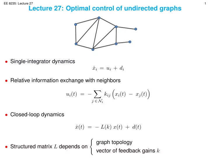
Draft EE 8235: Lecture 27 1 Lecture 27: Optimal control of undirected graphs • Single-integrator dynamics x i = u i + d i ˙ • Relative information exchange with neighbors � � � u i ( t ) = − k ij x i ( t ) − x j ( t ) j ∈ N i • Closed-loop dynamics x ( t ) = − L ( k ) x ( t ) + d ( t ) ˙ � graph topology • Structured matrix L depends on vector of feedback gains k

Draft EE 8235: Lecture 27 2 • Independent of graph topology and feedback gains L ( k ) 1 = 0 · 1 Average mode N 1 � x ( t ) = ¯ x i ( t ) : undergoes random walk N i = 1 If other modes are stable, x i ( t ) fluctuates around ¯ x ( t ) deviation from average: x i ( t ) = x i ( t ) − ¯ ˜ x ( t ) � � x T ( t ) ˜ steady-state variance: t → ∞ E lim ˜ x ( t )

Draft EE 8235: Lecture 27 3 Optimal control problem What graph topologies lead to small variance? How to design feedback gains to minimize variance? x ( t ) ˙ = − L ( k ) x ( t ) + d ( t ) � � � � 1 N 11 T I − x ( t ) ˜ z ( t ) = = x ( t ) u ( t ) − L ( k ) • Setup: ⋆ Undirected graphs: bi-directional interaction between nodes ⋆ Symmetric feedback gains L ( k ) = L T ( k ) k ij = k ji ⇒

Draft EE 8235: Lecture 27 4 Incidence matrix • Edge l ∼ ( i, j ) : connects nodes i and j ⋆ Define e l ∈ R N with only two nonzero entries ( e l ) i = 1 ( e l ) j = − 1 Incidence matrix: E = [ e 1 · · · e m ]   1 1 1   x 1 − x 2 − 1 0 0   E T x = E T 1 = 0  , E =  , x 1 − x 3    0 − 1 0  x 1 − x 4 0 0 − 1 Edge l ∼ ( i, j ) : k l := k ij = k ji m � L ( K ) = E K E T = k l e l e T Laplacian: l l = 1   k 1 ...   Structured feedback gain: K =   k m

Draft EE 8235: Lecture 27 5 Tree graphs • Trees: connected graphs with no cycles path star Incidence matrix of a tree E t ∈ R N × ( N − 1)   1 0 0 − 1 1 0   E t =   0 − 1 1   0 0 − 1   1 1 1 − 1 0 0   E t =   0 − 1 0   0 0 − 1

Draft EE 8235: Lecture 27 6 • Coordinate transformation � � � � � � E T ψ ( t ) ψ ( t ) � � t E t ( E T t E t ) − 1 = x ( t ) ⇔ x ( t ) = 1 x ( t ) ¯ x ( t ) ¯ 1 N 1 T � �� � T − 1 � �� � T In new coordinates � ˙ � � � � � E T � � � E T ψ ( t ) ψ ( t ) � t t E t K E T E t ( E T t E t ) − 1 = − + d ( t ) 1 ˙ t x ( t ) ¯ x ( t ) ¯ 1 1 N 1 T N 1 T � � � � � � E T − E T t E t K 0 ψ ( t ) t = + d ( t ) 0 0 x ( t ) ¯ 1 N 1 T � � � � � 1 N 11 T I − ψ ( t ) � E t ( E T t E t ) − 1 z ( t ) = 1 − E t K E T x ( t ) ¯ t

Draft EE 8235: Lecture 27 7 Tree graphs: structured optimal H 2 design ˙ − E T t E t K ψ ( t ) + E T ψ ( t ) = t d ( t ) � � E t ( E T t E t ) − 1 z ( t ) = ψ ( t ) − E t K H 2 norm (from d to z ) � � J ( K ) = 1 t E t ) − 1 K − 1 + KE T ( E T 2 trace t E t   k 1 ...   Diagonal matrix: K =   k N − 1 • Structured optimal feedback gains �� � − 1 E T t E t ii k i = , i = 1 , . . . , N − 1 2

Draft EE 8235: Lecture 27 8 • In Lecture 28, I made a blunder on board while deriving the optimal values of k i Here is correct derivation: � � − 1 � � − 1 E T E T ⋆ G := t E t ⇒ diagonal elements of G determined by G ii = t E t ii ⋆ All diagonal elements of E T t E t are equal to 2   e T 1 t E t = [ e 1 · · · e N − 1 ] T [ e 1 · · · e N − 1 ] = . E T   .  [ e 1 · · · e N − 1 ] .  e T N − 1     e T e T e T 1 e 1 · · · 1 e N − 1 2 · · · 1 e N − 1 . . . . ... ...     . . . . =  = . . . .    e T e T e T N − 1 e 1 · · · N − 1 e N − 1 N − 1 e 1 · · · 2 ⋆ K – diagonal matrix ⇒ J ( K ) can be written as N − 1 � G ii � � J ( K ) = + k i 2 k i i = 1 ⋆ J ( K ) in a separable form ⇒ element-wise minimization will do � � G ii � d = − G ii G ii + k i + 1 = 0 ⇒ k i = 2 , i = 1 , . . . , N − 1 2 k 2 d k i 2 k i i

Draft EE 8235: Lecture 27 9 Optimal gains for star and path � N − 1 1 • Star: uniform gain k = ≈ √ for large N 2 N 2 • Path: � i ( N − i ) k i = 2 N largest gains in the center

Draft EE 8235: Lecture 27 10 General undirected graphs • Decompose graph into a tree subgraph and remaining edges � E t � Incidence matrix: E = E c � − 1 E T � Π = E t E + E T = E t t E t Projection matrix: t t E c ∈ range (Π) : E c = Π E c       1 0 0 1 1 0 0 1 − 1 1 0 0 − 1 1 0 0        =  ∪       0 − 1 1 − 1 0 − 1 1 − 1     0 0 − 1 0 0 0 − 1 0 � E t � E t � � E = E c = Π E c � t E t ) − 1 E T � ( E T = E t I t E c = E t M

Draft EE 8235: Lecture 27 11 General graphs: structured optimal H 2 design t E t M K M T ψ ( t ) + E T ˙ − E T ψ ( t ) = t d ( t ) � � � � − 1 E T E t t E t z ( t ) = ψ ( t ) − E t M K M T tree graphs: M = I H 2 norm (from d to z ) � � � J ( K ) = 1 M K M T � − 1 + M K M T E T � − 1 � E T 2 trace t E t t E t • Main result: M K M T > 0 ⋆ Closed-loop stability ⇔ { W 1 > 0 , W 2 = W T 2 } then − W 1 W 2 Hurwitz ⇔ W 2 > 0 ⋆ M K M T > 0 ⇒ convexity of J ( K )

Draft EE 8235: Lecture 27 12 • Semi-definite program 1 � � X + M K M T E T minimize 2 trace t E t � � ( E T t E t ) − 1 / 2 X > 0 t E t ) − 1 / 2 ( E T M K M T subject to K diagonal • Use CVX to solve it cvx_begin sdp variable k(Ne) % vector of unknown feedback gains variable X(Nv-1,Nv-1) symmetric; X == semidefinite(Nv-1); % Schur complement variable Mk = M*diag(k)*M’; % Matrix Mk minimize(0.5*trace( q*X + r*Mk*W )) subject to [X, invWh; invWh, Mk] > 0; cvx_end

Draft EE 8235: Lecture 27 13 Examples • Compare with performance of uniform gain design J ∗ ( J − J ∗ ) /J ∗ J ( k = 1) 9 . 1050 13 . 1929 45%

Draft EE 8235: Lecture 27 14 • Analytical results for circle and complete graphs � N 2 − 1 ⋆ Circle uniform gain k = 24 N 2 ⋆ Complete graph uniform gain k = N

Draft EE 8235: Lecture 27 15 Additional material • Papers to read ⋆ Xiao, Boyd, Kim, J. Parallel Distrib. Comput. ’07 ⋆ Zelazo & Mesbahi, IEEE TAC ’11 ⋆ Lin, Fardad, Jovanovic, CDC ’10