SLIDE 15 Regressor'!"
15
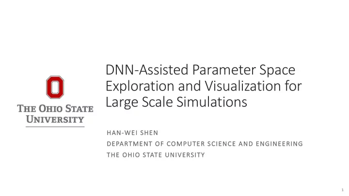
concat (1536, 4×4×16×k) reshape (k, 3, 3, 3) tanh
simulation parameters
(512) (l) (l, 512) (512, 512) (1536) (4×4×16×k) (4, 4, 16×k) (in=16×k, out=16×k) (in=16×k, out=8×k) (in=8×k, out=8×k) (in=8×k, out=4×k) (in=4×k, out=2×k) (in=2×k, out=k) (8, 8, 16×k) (16, 16, 8×k) (32, 32, 8×k) (64, 64, 4×k) (128, 128, 2×k) (256, 256, k) (256, 256, 3) image
ReLU
bacth normalization 2D convolution fully connected residual block
(in, out, 3, 3) (out, out, 3, 3) upsampling (in, out, 1, 1) upsampling sum
input/output view parameters
(512) (n) (n, 512) (512, 512)
visual mapping parameters
(512) (m) (m, 512) (512, 512)
a
- 2D%Convolutional%Layer
- Input:%tensor%# ∈ ℝ&×(×)
- Output:%tensor%* ∈ ℝ&×(×)+
- Weights:%kernel%, ∈
ℝ-_(×-_&×)×)+
- Residual%block1
- Adding%input%to%the%output%
- f%convolutional%layers
* = , ∗ #
1K.%He,%X.%Zhang,%S.%Ren,%and%J.%Sun.%Deep%residual%learning%for%image%recognition.%In%Proceedings%of%2016%IEEE%
Conference%on%Computer%Vision%and%Pattern%Recognition,%pp.%770–778,%2016.