DMD array Scene Lens1 A/D Photo diode Lens2 converter Ref: - - PowerPoint PPT Presentation

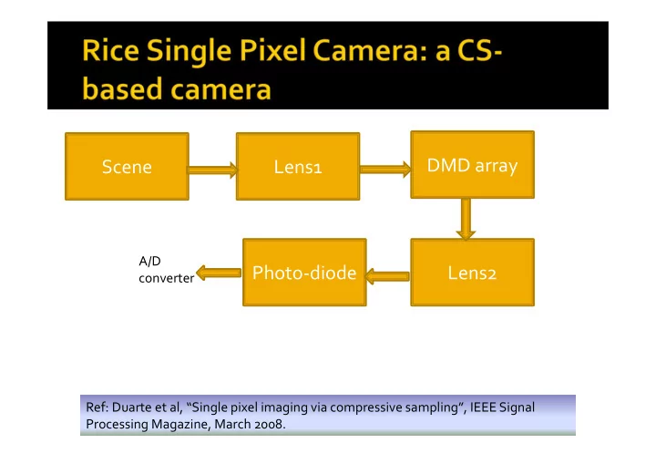
Ref: Duarte et al, “Single pixel imaging via compressive sampling”, IEEE Signal Processing Magazine, March 2008.

Scene Lens1 DMD array Lens2 Photo‐diode

A/D converter

 Contains no detector array.  Light from the scene passes through Lens1

and is focussed on a digital micromirror device (DMD).

 DMD is a 2D array of thousands of very tiny

mirrors.

 Light reflected from DMD passes through the

second lens and to the photodiode.

 These values {yi} are output in the form of a voltage which is

then digitized by an A/D converter.

 Note that a different binary code vector i is used for each yi,

1 <= i <= m.

 The random binary code is implemented by setting the

• rientation of the mirrors (facing toward or away from

Lens2) randomly within the hardware.

 But these are codes with 0 and 1 and such a matrix does not

• bey RIP.

 So instead a matrix with ‐1 and +1 is “generated” using two

measurements:

x y y x y x y ) (

2 1 2 1 2 2 1 1

        

Φ2 contains a 1 wherever Φ1 contains a 0, and Φ2 contains a 1 wherever Φ1 contains a 0.

 The basic measurement model can be written

as follows (in vector notation):

 As per CS theory, there are guarantees of

good reconstruction if the number of samples

• beys (for K‐sparse signals):

) ,..., , ( , ] | ... | | [ ,

2 1 m T

y y y    y φ φ φ Φ Φf y

m 2 1

)) / log( ( K n K O m 



   

x y y x f

y x f y x f f TV f y f TV ) , ( ) , ( ) ( that such ) ( min

2 2

Optimization technique used: Refer to reconstruction results in the following article: Duarte et al, “Single pixel imaging via compressive sampling”, IEEE Signal Processing Magazine, March 2008

More Results: http://dsp.rice.edu/cscamera

Original 4096 pixels, 800 measurements, i.e. 20% data

Informal description of Rice Single Pixel Camera: http://terrytao.wordpress.com/2007/04/13/compressed‐sensing‐ and‐single‐pixel‐cameras/



This is a compressive camera developed at Stanford, that uses the same mathematical model as the Rice SPC.



The difference is that it calculates all the m dot products on a single CMOS chip and simultaneously



What dot products? Of a random pattern (with a elements) with a vector of a n analog pixel values.



Only the m << n dot products are are quantized (Analog to digital conversion), saving huge amounts of energy.



Mounted on a mobile phone – led to 15 fold savings in battery power.



See here for more information.



Yields excellent quality reconstruction with high frame rates (960 fps).



Reason for being able to increase frame rate is that fewer measurements are made within each exposure time (m << n) than a conventional camera.

Image source: Oike and El‐Gamal, “CMOS sensor with programmable compressed sensing”, IEEE Journal of Solid State Electronics, January 2013 http://isl.stanford.edu/~abbas/papers/PDF1.pdf

Image source: Oike and El‐Gamal, “CMOS sensor with programmable compressed sensing”, IEEE Journal of Solid State Electronics, January 2013 http://isl.stanford.edu/~abbas/papers/PDF1.pdf

 SPC can be extended for video.  Consider a video with a total of F (2D) images, each

with n pixels.

 In the still‐image SPC, an image was coded several

times using different binary codes i where i ranges from 1 to M.

 Note that in a video‐camera, this reduces the video

frame rate.

 Assume we take a total of M measurements, i.e. M/F

measurements (dot products) per frame.

 We make the simplifying assumption that the scene

changes slowly or not at all within the set of M/F dot products.

 Method 1: To reconstruct the original video

from the CS measurements, we could use a 2D DCT/wavelet basis  and perform F independent (2D) frame‐by‐frame reconstructions, by solving:

 This procedure fails to exploit the tremendous

inter‐frame redundancy in natural videos.

F M n n n n F M

R R R R F t

/ / 1

, , , , that such min }, ,..., 1 {        

  t t t t t t t t t θ

y θ Ψ Φ Ψθ Φ f Φ y θ

t

 Method 2: Create a joint measurement matrix  for

the entire video sequence, as shown below.  is block‐diagonal, with each of the diagonal blocks being the matrix t for measurement yt at time t.

i i F 2 1

f y y y y y

i i F 2 1

Φ Φ Φ Φ Φ Φ Φ     

 

), | ... | | ( , ,

/ n F M Fn M

R R

 Method 2 (continued) : Use a 3D DCT/wavelet basis

 (size Fn by Fn) for sparse representation of the video sequence:

 Videos frames change slowly in time. The 3D‐

DCT/wavelet encourages smoothness in the time dimension.

M Fn Fn Fn Fn M

R R R R      

 

y θ Ψ Φ ΦΨθ Φf y θ

θ

, , , , such that min

1

 Method 3 (Hypothetical): Assume we had a 3D SPC

with a full 3D sensing matrix  which operates on the full video, and with an associated 3D wavelet/DCT basis.

 Unlike method 2,  is not block‐diagonal.  Also, such a scheme is not realizable in practice – as dot

products cannot be computed for an entire video.

 This method is purely for reference comparison.

M Fn Fn Fn Fn M

R R R R      

 

y θ Ψ Φ ΦΨθ Φf y θ

θ

, , , , that such min

1

 Experiment performed on a video of a moving

disk (against a constant background) ‐ size 64 x 64 with F = 64 frames.

 This video is sensed with a total of M

measurements with M/F measurements per frame.

 All three methods (frame‐by‐frame 2D, 2D

measurements with 3D reconstruction, 3D measurements with 3D reconstruction) compared for M = 20000 and M = 50000.

Source of images: Duarte et al, “Compressive imaging for video representation and coding”, http://www.ecs.umass.ed u/~mduarte/images/CSCa mera_PCS.pdf

Method 1 Method 2 Method 3

 Hyperspectral images are images of the form

M x N x L, where L is the number of channels. L can range from 30 to 30,000 or more.

 The visible spectrum ranges from ~420 nm to

~750 nm.

 Finer division of wavelengths than possible in

RGB!

 Can contain wavelengths in the infrared or

ultraviolet regime.

Multiple sensor arrays – one per wavelength. Expensive!

 Reconstruction of hyperspectral data imaged by

a coded aperture snapshot spectral imager (CASSI) developed at the DISP (Digitial Imaging and Spectroscopy) Lab at Duke University.

 CASSI measurements are a superposition of

aperture‐coded wavelength‐dependent data: ambient 3D hyperspectral datacube is mapped to a 2D ‘snapshot’.

 Task: Given one or more 2D snapshots of a

scene, recover the original scene (3D datacube).

Reference color image (only for reference – NOT acquired by the camera) Snapshot spectral image acquired by CASSI camera http://www.disp.duke.edu/projects/CASSI/experimentaldata/index.ptml

http://www.disp.duke.edu/projects/CASSI/exp erimentaldata/index.ptml

Ref: A. Wagadarikar et al, “Single disperser design for coded aperture snapshot spectral imaging”, Applied Optics 2008.

scene Lens Coded aperture Prism Detector array

A coded aperture is a cardboard/plastic piece with holes of small size etched in at random spatial

• locations. This simulates a binary mask. In some

cases, masks that simulate transparency values from 0 (full opaque) to 1 (fully transparent) can also be prepared.

“White” Light from ambient scene Coded aperture Prism Detector array

 Assume we want to measure a hyperspectral data‐

cube given as where data at each wavelength is a 2D image of size where the number of wavelength is .

 In a CASSI camera, each image , is

multiplied by the same known (random)binary code given as yielding an image



N N N

y x

R

 

 X

y x

N N 



N



N j   1 ,

j

X

y x N

N 

 } 1 , { C

. ˆ C X X

j j

 

 Let the pixel at location in image be

denoted as . The shifted version of is given as where denotes the shift in the pixels at wavelength

 The wavelength‐dependent shifts are

implemented by means of a prism in the CASSI camera, whereas modulation by the binary code is implemented by means of a mask.

) , ( y x

j

X ˆ

) , ( ˆ y x X j

) , ( ˆ y x X j

) , ( ˆ ) , ( y l x X y x S

j j j

 



j

l . ˆ , ,

ˆ

j j l l

j j j

  

 The measurement by the CASSI system is a single 2D

“snapshot” given as follows (superposition of coded data from all wavelengths):

 Due to the wavelength‐dependent shifts, the contribution

to M(x,y) at different wavelengths corresponds to a different spatial location in each of the slices of the datacube X.

 Also the portions of the coded aperture contributing

towards a single pixel value M(x,y) are different for different wavelengths.

) , ( ) , ( ) , ( ˆ ) , ( ) , (

1 1 1

y l x C y l x X y l x X y x S y x M

j N j j j N j j j N j j

      

  

  

  

• Aperture Code: created randomly (random binary, [0,1]

uniform random also possible)

• The aperture code pattern has holes of size 2 x 2 pixels

(smaller holes give rise to diffraction artifacts).

• The pattern is projected onto the detector array in a

magnified form.

• Note: Random mask pattern is needed as per CS theory.

 The compression rate of CASSI is the number of

wavelengths: 1.

 This compression rate can be reduced if T > 1

snapshots of the same scene are acquired in quick succession, denoted as reducing the compression rate to .

 Each snapshot is acquired using a different aperture

code, i.e. a different mask pattern ‐ implemented in hardware by moving the position of the mask using a piezo‐electric mechanism.

 Reduction in compression rate = less ill‐posed

problem = scope for better reconstruction.

T t 1

} {

 t

M

T N :



 A total‐variation based CS solver called as

TwIST was used (ref: Bioucas‐Dias and Figuereido, A

new twist: Two‐step iterative shrinkage/thresholding algorithms for image restoration”, IEEE Transactions on Image Processing, 2007.)  The inversion is performed by solving the

following:

 

  

        

x y

N x N y N t f

y x f y x f y x f y x f TV TV E

1 1 1 2 2 2

)) , , ( ) , 1 , ( ( )) , , ( ) , , 1 ( ( ) ( ), ( min ) (





     f f f Φ m f*

t t