Distinguishing strings From lecture 3: Definition Let L be language - PowerPoint PPT Presentation

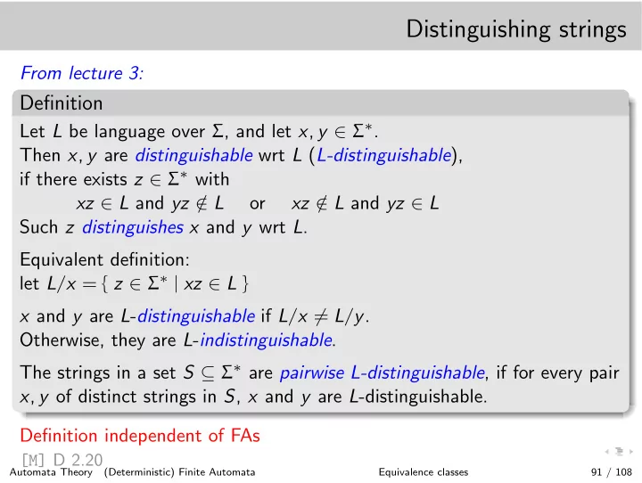
Distinguishing strings From lecture 3: Definition Let L be language over Σ , and let x , y ∈ Σ ∗ . Then x , y are distinguishable wrt L ( L-distinguishable ), if there exists z ∈ Σ ∗ with xz ∈ L and yz / ∈ L or xz / ∈ L and yz ∈ L Such z distinguishes x and y wrt L . Equivalent definition: let L / x = { z ∈ Σ ∗ | xz ∈ L } x and y are L - distinguishable if L / x � = L / y . Otherwise, they are L - indistinguishable . The strings in a set S ⊆ Σ ∗ are pairwise L-distinguishable , if for every pair x , y of distinct strings in S , x and y are L -distinguishable. Definition independent of FAs [M] D 2.20 Automata Theory (Deterministic) Finite Automata Equivalence classes 91 / 108

Equivalence relation R equivalence relation on A – reflexive xRx for all . . . – symmetric xRy then yRx – transitive xRy and yRz then xRz equivalence class [ x ] R = { y ∈ A | yRx } short: [ x ] partition A [M] Sect. 1.3 Automata Theory (Deterministic) Finite Automata Equivalence classes 92 / 108

Definition For a language L ⊆ Σ ∗ , we define the relation ≡ L (an equivalence relation) on Σ ∗ as follows: for x , y ∈ Σ ∗ if and only if x and y are L -indistinguishable x ≡ L y Equivalence relation. . . right invariant x ≡ L y implies xz 1 ≡ L yz 1 Book uses I L for ≡ L Automata Theory (Deterministic) Finite Automata Equivalence classes 93 / 108

Example L 1 = { x ∈ { a , b } ∗ | x ends with aa } L / x for x = Λ , a , b , aa . . . Equivalence classes / partitioning of { a , b } ∗ = { Λ , a , b , aa , ab , ba , bb , aaa , aab , aba , abb , baa , . . . } . . . Automata Theory (Deterministic) Finite Automata Equivalence classes 94 / 108

Example Equivalence classes of ≡ L , where L = AnBn = { a i b i | i � 0 } [M] E 2.37 Automata Theory (Deterministic) Finite Automata Equivalence classes 95 / 108

Example Equivalence classes of ≡ L , where L = AnBn = { a i b i | i � 0 } { Λ } , { a } , { a 2 } , { a 3 } , . . . { a i b i | i � 1 } { a i + 1 b i | i � 1 } , { a i + 2 b i | i � 1 } , { a i + 3 b i | i � 1 } , . . . { x ∈ { a , b } ∗ | x is not a prefix of any element of L } = { b , ba , bb , aba , abb , baa , . . . } Infinitely many equivalence classes quotients – L / a i = { a k b i + k | k � 0 } – L / a i + k b i = { b k } i > 0, k � 0 – L / a i b j = L / xbay = ∅ j > i [M] E 2.37 Automata Theory (Deterministic) Finite Automata Equivalence classes 96 / 108

Example L 1 = { x ∈ { a , b } ∗ | x ends with aa } L / x for x = Λ , a , b , aa . . . Equivalence classes / partitioning of { a , b } ∗ = { Λ , a , b , aa , ab , ba , bb , aaa , aab , aba , abb , baa , . . . } : { Λ , b , ab , bb , aab , abb , . . . } { a , ba , aba , . . . } { aa , aaa , baa , . . . } Finitely many equivalence classes Automata Theory (Deterministic) Finite Automata Equivalence classes 97 / 108

x ends with aa From lecture 1: Example L 1 = { x ∈ { a , b } ∗ | x ends with aa } b a a a q 0 q 1 q 2 b b [M] E. 2.1 Automata Theory (Deterministic) Finite Automata Equivalence classes 98 / 108

L q = { x ∈ Σ ∗ | δ ∗ ( q 0 , x ) = q } State q in FA ≈ From lecture 3: Theorem Suppose M = ( Q , Σ , q 0 , A , δ ) is an FA accepting L ⊆ Σ ∗ . If x , y ∈ Σ ∗ are L-distinguishable, then δ ∗ ( q 0 , x ) � = δ ∗ ( q 0 , y ) . For every n � 2 , if there is a set of n pairwise L-distinguishable strings in Σ ∗ , then Q must contain at least n states. Proof. . . [M] Thm 2.21 In other words: if δ ∗ ( q 0 , x ) = δ ∗ ( q 0 , y ) , then x , y are L -indistinguishable. Each L q is subset of equivalence class Automata Theory (Deterministic) Finite Automata Equivalence classes 99 / 108

Myhill-Nerode Theorem If L ⊆ Σ ∗ can be accepted by a finite automaton, then the set Q L of equivalence classes of the relation ≡ L is finite. Conversely, if the set Q L is finite, the finite automaton M L = ( Q L , Σ , q 0 , A , δ ) accepts L, where q 0 = [ Λ ] A = { q ∈ Q L | q ⊆ L } δ ([ x ] , σ ) = [ x σ ] Finally, M L has the fewest states of any FA accepting L. Note: If x ∈ L , then [ x ] ⊆ L ( L is union of equivalence classes) Right invariant x ≡ L y implies x σ ≡ L y σ [M] Thm 2.36 Automata Theory (Deterministic) Finite Automata Equivalence classes 100 / 108

From lecture 3: Theorem For every language L ⊆ Σ ∗ , if there is an infinite set S of pairwise L-distinguishable strings, then L cannot be accepted by a finite automaton. Proof. . . [M] Thm 2.26 Automata Theory (Deterministic) Finite Automata Equivalence classes 101 / 108

Minimizing states ALGORITHM mark pairs of non-equivalent states start by marking pairs ( p , q ) where exactly one p , q in A repeat for each unmarked pair ( p , q ) check whether there is a σ such that ( δ ( p , σ ) , δ ( p , σ ) ) is marked then mark ( p , q ) until this pass does not mark new pairs a 1 a 2 a k × k − 1 × k × 0 × 1 × 2 a 1 a 2 a k [M] Algo 2.40 Automata Theory (Deterministic) Finite Automata Minimization 102 / 108

b a b 1 2 0 1 2 2 2 . a a a a b 3 1 1 1 b b b 4 1 1 1 . 9 8 3 4 5 2 . . 1 1 a a a a b 6 2 2 2 1 1 2 6 7 2 2 2 1 1 2 . 7 5 b a 8 1 1 1 . . 1 1 1 9 1 1 1 2 3 1 1 1 2 b b 0 1 2 3 4 5 6 7 8 Resulting (minimal) FA. . . [M] Fig 2.42 Automata Theory (Deterministic) Finite Automata Minimization 103 / 108

b b a b 0 1 2 5 b b a a a a a a b b b b 9 8 3 4 a 7 6 b a a b a 1,2,5 0 b a a b b 8,3,4 9 a 7,6 b a [M] Fig 2.42 Automata Theory (Deterministic) Finite Automata Minimization 104 / 108

⊠ Example: Brzozowski minimization a a a a 1 2 1 2 a a b b ǫ ǫ b b b b b b b b 3 4 3 4 a a a a last a (odd b ) a 123 a a a , b ǫ 124 ǫ 1234 1 2 a , b a b b b b b b 23 124 34 ǫ 12 3 4 b b b a a even b a a a Automata Theory (Deterministic) Finite Automata Minimization 105 / 108

above Brzozowski observes that one can minimize an FA by performing the following operations twice: invert (mirror), then determinize. It is rather magical that this indeed works. The method is in theory rather unfavourable, because of the exponentiation when detrminizing, but in practice seems not too slow.

b b a b 0 1 2 5 b L = L ( M ) b a a a a a a b b b b 9 8 3 4 a state δ ∗ ( q 0 , x ) ≡ M 7 6 ≡ L “future” L / x b a a x ≡ M y , then x ≡ L y . b Σ ∗ a 1,2,5 0 b a a b b 8,3,4 9 a 7,6 b a [M] Fig 2.42 Automata Theory (Deterministic) Finite Automata Minimization 106 / 108

Distinguishing states From lecture 3: L = { aa , aab } ∗ { b } q 0 a b a , b b p s r a a , b a a b u t b [M] E 2.22 Automata Theory (Deterministic) Finite Automata Minimization 107 / 108

Distinguishing states L = { aa , aab } ∗ { b } L /σ = { z ∈ Σ ∗ | σ z ∈ L } L σ [ x ] σ → L /σ → [ x σ ] L { aa , aab } ∗ { b } { a , ab } L a b [ Λ ] a , b b { a , ab }{ aa , aab } ∗ { b } { Λ } ∅ a b a , b b a [ a ] [ ab ] [ b ] a , b a a b a a , b { Λ , b }{ aa , aab } ∗ { b } { aa , aab } ∗ { b } ∪ { Λ } a a b b [ aa ] [ aab ] L ∪ { b } L L ∪ { Λ } b [M] E 2.22 see ֒ → E 3.6 Automata Theory (Deterministic) Finite Automata Minimization 108 / 108