Direct and Partial Variation MPM1D: Principles of Mathematics Recap - - PDF document

p r o p e r t i e s o f l i n e a r r e l a t i o n s

MPM1D: Principles of Mathematics

First Differences

• J. Garvin

Slide 1/15

p r o p e r t i e s o f l i n e a r r e l a t i o n s

Direct and Partial Variation

Recap

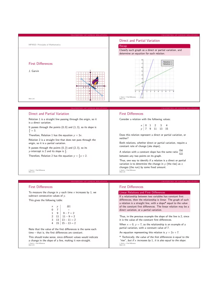
Classify each graph as a direct or partial variation, and determine an equation for each relation.

• J. Garvin — First Differences

Slide 2/15

p r o p e r t i e s o f l i n e a r r e l a t i o n s

Direct and Partial Variation

Relation 1 is a straight line passing through the origin, so it is a direct variation. It passes through the points (0, 0) and (1, 3), so its slope is

3 1 = 3.

Therefore, Relation 1 has the equation y = 3x. Relation 2 is a straight line that does not pass through the

• rigin, so it is a partial variation.

It passes through the points (0, 2) and (2, 3), so its y-intercept is 2 and its slope is 1

2.

Therefore, Relation 2 has the equation y = 1

2x + 2.

• J. Garvin — First Differences

Slide 3/15

p r o p e r t i e s o f l i n e a r r e l a t i o n s

First Differences

Consider a relation with the following values: x 1 2 3 4 y 7 9 11 13 15 Does this relation represent a direct or partial variation, or neither? Both relations, whether direct or partial variation, require a constant rate of change (aka slope). A relation with a constant slope has the same ratio rise run between any two points on its graph. Thus, one way to identify if a relation is a direct or partial variation is to determine the change in y (the rise) as x changes (the run) by some fixed amount.

• J. Garvin — First Differences

Slide 4/15

p r o p e r t i e s o f l i n e a r r e l a t i o n s

First Differences

To measure the change in y each time x increases by 1, we subtract consecutive values of y. This gives the following table: x y ∆1 7 – 1 9 9 − 7 = 2 2 11 11 − 9 = 2 3 13 13 − 11 = 2 4 15 15 − 13 = 2 Note that the value of the first differences is the same each time – that is, the first differences are constant. This should make sense, since different values would indicate a change in the slope of a line, making it non-straight.

• J. Garvin — First Differences

Slide 5/15

p r o p e r t i e s o f l i n e a r r e l a t i o n s

First Differences

Linear Relations and First Differences

If a relationship between two variables has constant first differences, then the relationship is linear. The graph of such a relation is a straight line, with a slope* equal to the value

• f the constant first differences. The linear relation may be a

direct variation, or a partial variation. Thus, in the previous example the slope of the line is 2, since it is the value of the constant first differences. When x = 0, y = 7, so the relationship is an example of a partial variation, with a constant value of 7. An equation representing this relation is y = 2x + 7. * Technically, the value of the first differences is equal to the “rise”, but if x increases by 1, it is also equal to the slope.

• J. Garvin — First Differences

Slide 6/15

p r o p e r t i e s o f l i n e a r r e l a t i o n s

First Differences

A graph of the relation confirms that it is linear, and a partial variation.

• J. Garvin — First Differences

Slide 7/15

p r o p e r t i e s o f l i n e a r r e l a t i o n s

First Differences

Example

Classify the relation below as linear or non-linear. x 1 2 3 4 y 8 15 22 29 36 Since x increases by the same amount, find the first differences. x y ∆1 8 – 1 15 15 − 8 = 7 2 22 22 − 15 = 7 3 29 29 − 22 = 7 4 36 36 − 29 = 7

• J. Garvin — First Differences

Slide 8/15

p r o p e r t i e s o f l i n e a r r e l a t i o n s

First Differences

Since we obtain the same value, 7, for the first differences, the relation is linear.

• J. Garvin — First Differences

Slide 9/15

p r o p e r t i e s o f l i n e a r r e l a t i o n s

First Differences

Example

Classify the relation below as linear or non-linear. x 1 2 3 4 y 3 5 11 21 35 Since x increases by the same amount, find the first differences. x y ∆1 3 – 1 5 5 − 3 = 2 2 11 11 − 5 = 6 3 21 21 − 11 = 10 4 35 35 − 21 = 14

• J. Garvin — First Differences

Slide 10/15

p r o p e r t i e s o f l i n e a r r e l a t i o n s

First Differences

Since we obtain different first difference values, the relation is non-linear.

• J. Garvin — First Differences

Slide 11/15

p r o p e r t i e s o f l i n e a r r e l a t i o n s

First Differences

Example

Classify the relation below as linear or non-linear. If it is linear, determine an equation for the relation. x 2 4 6 8 y 15 11 7 3 Begin by determining the first differences. x y ∆1 2 15 – 4 11 11 − 15 = −4 6 7 7 − 11 = −4 8 3 3 − 7 = −4 The first differences are constant, indicating a linear relation.

• J. Garvin — First Differences

Slide 12/15

p r o p e r t i e s o f l i n e a r r e l a t i o n s

First Differences

This scenario is different for a few reasons. The value of the finite differences is negative, indicating that the relation has a negative slope. While x increases by the same amount, it increases by 2 each time instead of 1. This means the “run” of our slope will be 2, rather than 1. Since the value of the finite differences is equal to the “rise”

• f our slope, the slope is − 4

2 = −2.

The table of values begins at x = 2, rather than x = 0, so we will need to work backward to find the constant value if it is a partial variation.

• J. Garvin — First Differences

Slide 13/15

p r o p e r t i e s o f l i n e a r r e l a t i o n s

First Differences

The y-values of the relation decrease by 4 for each increase

• f 2 in x.

If we go backward and decrease x by 2, we need to increase y by 4 instead. Thus, when x = 0, y = 15 + 4 = 19. Therefore, an equation for the linear relation is y = −4x + 19.

• J. Garvin — First Differences

Slide 14/15

p r o p e r t i e s o f l i n e a r r e l a t i o n s

Questions?

• J. Garvin — First Differences

Slide 15/15