Detecting Geoneutrinos Giorgio Gratta Physics Dept Stanford - - PowerPoint PPT Presentation

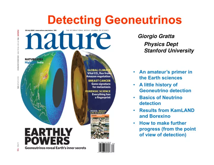
Detecting Geoneutrinos

Giorgio Gratta Physics Dept Stanford University

• An amateur’s primer in

the Earth sciences

• A little history of

Geoneutrino detection

• Basics of Neutrino

detection

• Results from KamLAND

and Borexino

• How to make further

progress (from the point

• f view of detection)

FROST, Fermilab, Mar 2016 G.Gratta - Geoneutrinos 2

Structure of the Earth: a particle physicist’s view

• From seismic data

5 basic regions:

• inner core,
• outer core,
• mantle,
• oceanic crust,
• continental

crust and sediments

• All these regions

behave like solids except the outer core.

Image by: Colin Rose and Dorling Kindersley

6400km 2900km 2255km 1245km 6km 35km

FROST, Fermilab, Mar 2016 G.Gratta - Geoneutrinos 3

Convection in the Earth

• The mantle appears to convect even though it is solid.
• This is responsible for plate tectonics and earthquakes.
• Oceanic crust is being renewed at mid-ocean ridges and

recycled at trenches.

Image: http://www.dstu.univ-montp2.fr/PERSO/bokelmann/convection.gif

FROST, Fermilab, Mar 2016 G.Gratta - Geoneutrinos 4

“Unwary readers should take warning that

• rdinary language undergoes modification to

a high-pressure form when applied to the interior of the Earth. A few examples of equivalents follow:

Francis Birch

• J. Geophys. Res. 57 (1952) 227

High-pressure form Ordinary meaning

certain dubious undoubtedly perhaps positive proof vague suggestion unanswerable argument trivial objection pure iron uncertain mixture of all the elements

FROST, Fermilab, Mar 2016 G.Gratta - Geoneutrinos 5

Very specific data on the Earth’s interior is hard to collect

Historically, the only universal probe for the interior

• f the Earth has been seismology.

 But this is only sensitive to the elastic properties of the rocks. Nomenclature derives from the seismic boundaries. Composition is then guessed for the different regions that are assumed homogeneous in composition. Seismically motivated nomenclature is then used at times to signify a region of a certain composition. This is sometimes confusing.

FROST, Fermilab, Mar 2016 G.Gratta - Geoneutrinos 6

OK, let’s say that the Earth probably has the same composition as the Solar System  How to average over the Solar System?

McDonough, Neutrino 2008

FROST, Fermilab, Mar 2016 G.Gratta - Geoneutrinos 7

C1 chondrites have very similar composition to the solar photosphere (except for peculiar light elements that are expected to be anomalous around the Sun)

McDonough, Neutrino 2008

FROST, Fermilab, Mar 2016 G.Gratta - Geoneutrinos 8

Next: 1) Correct for the loss of volatile elements during the Earth’s formation 2) Based on chemical affinity estimate the composition

• f different regions

 Core expected to have insignificant U, Th  Independently know that U, Th are ~1000x more common in the crust (ppm) than in the mantle (ppb)

McDonough, Neutrino 2008

Relative Abundance

FROST, Fermilab, Mar 2016 G.Gratta - Geoneutrinos 9

Only a shallow layer has been sampled for chemical composition by drilling/sampling

• Deepest bore-hole (12km) is only ~1/500 of the Earth’s radius
• Oceans and southern hemisphere substantially less studied

FROST, Fermilab, Mar 2016 G.Gratta - Geoneutrinos 10

Q: What powers the Eyjafjallajökull?

…more generally what powers plate tectonics and hence volcanoes?

FROST, Fermilab, Mar 2016 G.Gratta - Geoneutrinos 11

Same boreholes can be used to measure the heat flow from the Earth’s interior

• ∆Thole is measured between 2 points far away along

the borehole

• Thermal conductivity Crock of the rock is measured

in the lab

• Q = ∆Thole Crock (assuming pure conduction)
• But in addition have to account for mantle convection
• Get a total 463 TW (100 mW/m2)
• Error is small BUT other analyses with different

convection model gives 311 TW (61mW/m2)…

FROST, Fermilab, Mar 2016 G.Gratta - Geoneutrinos 12 Image: Pollack et. al

Heat flow from the Earth

Note the large emission under the mid ocean ridges (~83% of the total heat!): this is where mantle convects and this is also where the pure conduction model really does not work well.

FROST, Fermilab, Mar 2016 G.Gratta - Geoneutrinos 13 Image: Pollack et. al

From the Sun the Earth receives

• n average

1400W/m2 at the top of the atmosphere and 400W/m2 at the surface  the surface temperature has nothing to do with the heath produced inside.

Putting in context the 31-46TW produced by the planet

We need 15 TW to run human society. This is sizeable compared to the total output from the planet!

FROST, Fermilab, Mar 2016 G.Gratta - Geoneutrinos 14

Radiogenic heat / Total heat called “Urey ratio”  believed to be 0.3 to 0.7

What produces the heat ?

FROST, Fermilab, Mar 2016 G.Gratta - Geoneutrinos 15

The 238U long decay chain including β- decays

234Th

24.1d

238U

4.5Gyr

210Bi

5d

210Pb

22yr

214Po

0.16ms

214Bi

20m

214Pb

27m

218Po

3.0m

222Rn

3.8d

226Ra

1.6kyr

230Th

77kyr

234U

0.4Myr

234Pa

1.17min

206Pb

Stable

210Po

138d

β α α α α α α α α β β β β β

FROST, Fermilab, Mar 2016 16

The 232Th long decay chain including β- decays

α α α

0.64

β β β β β

232Th

14Gyr

208Pb

Stable

212Po

0.3μs

212Bi

61m

212Pb

11h

216Po

0.15s

220Rn

56s

224Ra

3.7d

228Th

1.9yr

228Ac

6.2h

228Ra

5.8yr

208Tl

3.1m 0.36

α α α α

G.Gratta - Geoneutrinos

The 40K β- decay

β

40Ca

Stable

40K

1.3Gy 0.89

40Ar

Stable

EC

0.11

FROST, Fermilab, Mar 2016 G.Gratta - Geoneutrinos 17

νe of different endpoint energy are emitted at each β- decay step producing characteristic spectra for

238U, 232Th (and 40K)

FROST, Fermilab, Mar 2016 G.Gratta - Geoneutrinos 18

…in the context of the other natural neutrinos…

K.Scholberg, Neutrino2014

~104

FROST, Fermilab, Mar 2016 G.Gratta - Geoneutrinos 19

Pre-history of Geoneutrinos

Fred Reines (?) working at a neutrino detector (circa 1953)

FROST, Fermilab, Mar 2016 G.Gratta - Geoneutrinos 20

…Well… not quite ! That detector was some 5 orders of magnitude too small

~30 TW

FROST, Fermilab, Mar 2016 G.Gratta - Geoneutrinos 21

Fast forward 45 years…

FROST, Fermilab, Mar 2016 G.Gratta - Geoneutrinos 22

GeoNeutrino Timeline

Pre-history: F.Reines’ & G.Gamov’s correspondence (1953) Early ideas: G.Eder, Nucl. Phys. 78 (1966) 657 G.Marx, Czech. J. Phys. B19 (1969) 1471 L.M.Krauss, S.L.Glashow, D.M.Schramm, Nature 310 (1984) 191 KamLAND proposal: P.Alivisatos et al, Stanford-HEP-98-03, Tohoku-RCNS-98-15 (1998) First experimental study (KamLAND): T.Araki et al., Nature 436 (2005) 499 Borexino enters the scene: G.Bellini et al. Phys. Lett. B687 (2010) 299 Latest KamLAND and Borexino results: A.Gando et al. (KamLAND), Phys. Rev. D 88 (2013) 033001 M.Agostini et al. (Borexino), Phys. Rev. D 92 (2015) 031101(R) …in addition there is now ample literature about the interpretation of the measurements (see later)

Neutrino-Signal Angle relative to Sun

The process can be used to point at the Sun!

FROST, Fermilab, Mar 2016 G.Gratta - Geoneutrinos 23

FROST, Fermilab, Mar 2016 G.Gratta - Geoneutrinos 24

νe e+

γ 511 keV γ 511 keV

n

γ 2200 keV

Large scintillator vat

10-40 keV

Eν measurement

 

    

e p n n e

m M M E E E ) (

 1800 keV

The process has a 1.8MeV threshold:  most of the flux is not accessible (no 40K)

FROST, Fermilab, Mar 2016 G.Gratta - Geoneutrinos 25

FROST, Fermilab, Mar 2016 G.Gratta - Geoneutrinos 26

FROST, Fermilab, Mar 2016 G.Gratta - Geoneutrinos 27

FROST, Fermilab, Mar 2016 G.Gratta - Geoneutrinos 28

FROST, Fermilab, Mar 2016 G.Gratta - Geoneutrinos 29

 Use inverse beta decay in liquid scintillator

Artificial reactors are a nuisance as the spectrum partially overlaps

Geoneutrinos are contained in the low energy part of the spectrum.

FROST, Fermilab, Mar 2016 G.Gratta - Geoneutrinos 30

Nuclear reactors traditionally have been a substantial “background” to the Geoneutrino measurement in KamLAND

After the Fukushima accident this background has gone away

KamLAND

0.9-2.6MeV time history Reactor only Reactor + backgrounds Reactor + Backgrounds +GeoNu model

FROST, Fermilab, Mar 2016 G.Gratta - Geoneutrinos 31

In order to help science and facilitate the study of GeoNeutrinos, Italy decided not to build new nuclear power plants and shut down the few they had!

FROST, Fermilab, Mar 2016 G.Gratta - Geoneutrinos 32

GeoNeutrinos

Borexino GeoNu data is cleaner but statistics not as good as KamLAND (smaller detector)

M.Agostini et al., Phys. Rev. D 92 (2015) 031101(R)

Null hypothesis excluded (3.6x10-9 or 5.9σ)

FROST, Fermilab, Mar 2016 G.Gratta - Geoneutrinos 33

2

4 ) ( ) , ( L L a L d L E dE dn A dE d     







  

The geo-neutrino flux due to a particular isotope accumulated at a particular position can be calculated as

Where:

• is the decay rate per unit mass for the isotope decay chain
• is the anti-neutrino energy spectrum for the decay chain
• is a correction accounting for neutrino oscillations
• is the amount of isotope at position

So from the measurement of the amount of isotope can be extracted by inverting this relationship The integral over the volume of the Earth introduces substantial degeneracy for a measurement done at a single site.

L 

dE dn /

A ) , ( L E 



 ) (L a  dE d /  ) (L a  L 

FROST, Fermilab, Mar 2016 G.Gratta - Geoneutrinos 34

So, for the time being we’ll use the flux measured at 2 sites to test models of U and Th distributions

A number of models have been developed over the last few years:

• R.S. Raghavan et al. Phys. Rev. Lett. 80 (1998) 635.
• C. Rothschild et al. Geo. Res. Lett. 25 (1998) 1083.
• F. Mantovani et al. Phys. Rev. D 69 (2004) 013001.
• G. Fiorentini et al. Phys. Rev. D 72 (2005) 033017.
• K.A. Hochmuth, Prog. Part. Nucl. Phys. 57 (2006) 293.
• G.L. Fogli et al. Earth, Moon, and Planets 99 (2007) 111.
• G. Fiorentini et al., Phys. Rep. 453 (2007) 117.
• S. Enomoto et al. Earth Planet. Sci. Lett. 258 (2007) 147.
• G. Fiorentini, et al., Phys. Rev. D 86 (2012) 033004.
• Y. Huang, et al., Geochem., Geophys., Geosyst. 14 (2013) 2003.
• O. Šramek, et al., Earth Planet. Sci. Lett. 361 (2013) 356.

Aside from the “interesting” part of estimating the global distributions of U and Th in core, mantle, continental and oceanic crusts, models require a more mundane, hi res description of the distributions in the nearby crust (because of the 1/L2 in the integral)

FROST, Fermilab, Mar 2016 G.Gratta - Geoneutrinos 35

~events/kton/yr Note the rate scale: in most places expect 4 events/month in a 1kton detector!

The expected rate at different world locations

FROST, Fermilab, Mar 2016 G.Gratta - Geoneutrinos 36

Background from reactors. Note that in many locations this is a severe problem (although reactors are off today in Japan)

FROST, Fermilab, Mar 2016 G.Gratta - Geoneutrinos 37

The ideal location to study the Earth’s mantle is the middle of an ocean, where there are no reactors and the crust is thinnest and depleted of Th & U

FROST, Fermilab, Mar 2016 G.Gratta - Geoneutrinos 38

But the uncertainty is still large and this is compatible with the C1 chondritic meteorite ratio mass ratio=3.9

In principle data could derive the Th/U ratio

Borexino

1σ 3σ 2σ

FROST, Fermilab, Mar 2016 G.Gratta - Geoneutrinos 39

Borexino flux (TNU) KamLAND flux (TNU) Local crust (local geology) Remote crust (global property) Total crust Continental Lithospheric Mantle (Homogeneous) Mantle Total model Measurement 1 TNU = 1 interaction/(yr 1032 target protons) ~ 1 interaction/(yr kton) For 232Th: Flux[10-6 cm-2s-1] = Rate[TNU]/4.07

238U: Flux[10-6 cm-2s-1] = Rate[TNU]/12.8

from L.Ludhova and S.Zavatarelli, arXiv:1310.3961 (15 Oct 2013)

How does the model compare with data for the total U + Th rates?

FROST, Fermilab, Mar 2016 G.Gratta - Geoneutrinos 40

 With the U/Th fixed by Chondritic Meteorites

from L.Ludhova and S.Zavatarelli, arXiv:1310.3961 (15 Oct 2013)

Crustal contributions Continental lithospheric mantle Remaining mantle contributions From PRD 92 (2015) 031101(R) Borexino claims detection of mantle neutrinos @98% CL (relies on crust models)

FROST, Fermilab, Mar 2016 G.Gratta - Geoneutrinos 41

The experiments start having some ability of discriminating between Earth models (and, for the time being, they pull in different directions)

KamLAND: PRD 88 (2013) 033001 Borexino: PRD 92 (2015) 031101

FROST, Fermilab, Mar 2016 G.Gratta - Geoneutrinos 42

The near future:

~1kton SNO site

FROST, Fermilab, Mar 2016 G.Gratta - Geoneutrinos 43

Slightly later: JUNO 20 kton liquid scintillator (~20x KamLAND ~60x Borexino!)

Hong Kong

FROST, Fermilab, Mar 2016 G.Gratta - Geoneutrinos 44

Steve Dye, AAP-2012, Honolulu Oct 2012

Of course the ideal site is oceanic (thinnest crust) Predicted Signals: Mid Pacific detector

FROST, Fermilab, Mar 2016 G.Gratta - Geoneutrinos 45

A 10kton dedicated detector that can be deployed in the ocean

FROST, Fermilab, Mar 2016 G.Gratta - Geoneutrinos 46

(my) wish list:

• Better statistics (larger detectors)
• Oceanic site
• Multiple sites
• Pointing ability
• Lower threshold (40K)

FROST, Fermilab, Mar 2016 G.Gratta - Geoneutrinos 47

Liquid scintillator technology is a limiting factor With more light one may be able to image events A typical organic scintillator (eg liquid scintillator) has energy efficiency of few% (~1 photon/100eV). Very hard to imagine doing much better.  Maybe energy can be stored in a material and its release triggered by ionization  Maybe ionized trails can produce fluorescent sites, then imaged …tried and failed, until now

FROST, Fermilab, Mar 2016 G.Gratta - Geoneutrinos 48

Liquid scintillator technology is a limiting factor If water-based was possible everything would be cheaper/larger (liquid scintillators were invented in the 30’s and are amazingly subtle/sophisticated things!)

FROST, Fermilab, Mar 2016 G.Gratta - Geoneutrinos 49

Photodetector technology is a limiting factor Photomultiplier Tubes (PMTs) are:

Bulky Clumsy/delicate (vacuum) Radioactive (glass) Small/non-scalable Expensive Low quantum efficiency devices

(PMTs were invented in the 30’s and are amazingly subtle/sophisticated things!)

FROST, Fermilab, Mar 2016 G.Gratta - Geoneutrinos 50

Concluding…

• KamLAND and Borexino will continue taking data (for a while), but

statistics accumulates linearly with time, further improvements are painful (the reactor-off period in Japan helps)

• SNO+ and JUNO will happen (“for free”)
• JUNO will be quite a bit larger than anything else:

will probably be the next highlight of the field …and then…

• Hanohano should happen, it is “just matter of money”
• Beyond this we are lacking the technology to make

further progress:

– Should do R&D on scintillators – Should do R&D on photodetectors

FROST, Fermilab, Mar 2016 G.Gratta - Geoneutrinos 51