Density Estimation Parametric techniques Maximum Likelihood - PDF document
1 Density Estimation Parametric techniques Maximum Likelihood Maximum A Posteriori Bayesian Inference G aussian M ixture M odels (GMM) EM-Algorithm Non-parametric techniques Histogram Parzen Windows
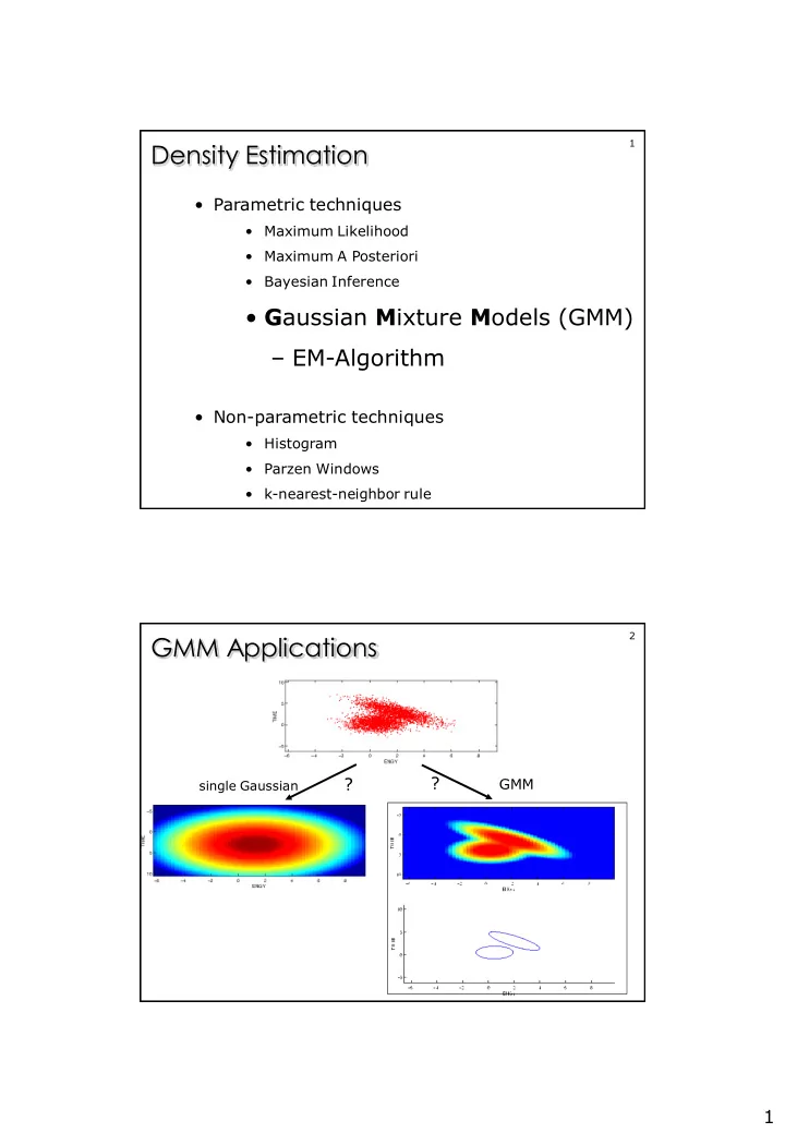
1 Density Estimation • Parametric techniques • Maximum Likelihood • Maximum A Posteriori • Bayesian Inference • G aussian M ixture M odels (GMM) – EM-Algorithm • Non-parametric techniques • Histogram • Parzen Windows • k-nearest-neighbor rule 2 GMM Applications ? GMM single Gaussian ? 1
3 GMM Applications Density estimation Observed data from a complex but unknown probability distribution. Can we describe this data with a few parameters ? Which (new) samples are unlikely to come from this unknown distribution (Outlier detection )? 4 GMM Applications Clustering Observations from K classes. Each class produces samples from a multivariate normal distribution. Which observations belong to which class ? Sometimes Sometimes Often possible easy impossible but not clear-cut 2
5 GMM: Definition • Mixture models are linear combinations of densities: K p x ( | ) c p x ( | ) i i i 1 K with c 1 , p x ( | ) dx 1 i i i 1 x – Capable of approximating almost any complex and irregularly shaped distributions ( K might get big )! • For Gaussian mixtures: { , }, ( | p x ) N ( , ) i i i i i i 6 Sampling a GMM • How to generate a random variable according to a K c N known GMM ( ) p x ( , ) i i i i Assume that each data point is generated according to the following recipe: 1. Pick a component ( i [ 1 .. K ] ) at random. Choose component i with probability c i . 2. Sample data point ~ N( i , i ) . In the end, we might not know which data points came from which component (unless someone kept track during the sampling process)! 3
7 Learning a GMM Recall ML-estimation We have: A density function p( · ; ) governed by a set of unknown parameters . A data set of size N drawn from this distribution X= { x 1 , ..., x N } We wish: to obtain the parameters best explaining data X by maximizing the log-likelihood function: L( ) ln p(X; ) argmax L( ) 8 Learning a GMM • For a single Gaussian distribution this is simple to solve. We have an analytical solution. • Unfortunately for many problems (including GMM) it is not possible to find analytical expressions. Resort to classical optimization techniques ? Possible but there is a better way: EM – Algorithm (Expectation-Maximization) 4
9 Expectation Maximization ( EM ) • General method for finding ML-estimates in the case of incomplete or missing data (GMM’s are one application). • Usually used when: • the observation is actually incomplete; some values are missing from the data set. • the likelihood function is analytically intractable but can be simplified by assuming the existence of additional but missing (so-called hidden/latent) parameters. The latter technique is used for GMMs. Think of each data point as having a hidden label specifying the component it belongs to. These component labels are the latent parameters. 10 General EM procedure The EM setting Observed data set ( incomplete ): X Assume a complete data set exists: Z = (X, Y) Z has a joint density function: p ( | ) p ( , | ) p ( | , ) p ( | ) y x x z x y Define the complete-data log-likelihood function: L( | ) L( | X,Y) ln (X,Y| p ) Our aim is to find a that maximizes this function. 5
11 General EM procedure • But: We cannot simply maximize L( | X,Y) ln p(X,Y| ) because Y is not known. • L ( |X, Y ) is in fact a random variable: - Y can be assumed to come from some distribution f ( | X, ) y That is, L ( |X, Y ) can be interpreted as a function where - X and are constant and Y is a random variable. • The EM will compute a new, auxiliary function, based on L , that can be maximized instead . • Let‘s assume we already have a reasonable estimate for the parameters: (i-1) . 12 General EM procedure • EM uses an auxiliary function: | ( i 1) ( i 1) Q ( , ) E ln (X,Y | p ) X, How to read this: – X and (i-1) are constants, – is a simple variable (the function argument), – Y is a random variable governed by distribution f . • The task is to rewrite Q and perform some calculations to make it a fully determined function. • Q is the expected value of the complete-data log-likelihood w.r.t. to missing data ( Y ), observed data ( X ) and current parameter estimates ( (i-1) ). This is called the E-step ( expectation-step ) 6
13 General EM procedure • Q can be rewritten by means of the marginal distribution f : If y is a continuous random variable: | ( i 1) ( i 1) Q ( , ) E ln (X,Y | p ) X, ( i 1) ln (X, p | ) f ( | X, ) dy y y Think of this as the expected y value of a function of Y If y is a discrete random variable: E[g(Y)] | ( i 1) ( i 1) Q ( , ) E ln (X,Y | p ) X, ( i 1) ln (X, p | ) ( | X, f ) y y y Evaluate f ( y | X, (i-1) ) , using the current estimate (i-1) . Now Q is fully determined and we can use it! 14 General EM procedure • In a second step Q is used to obtain a better set of parameters : ( ) i ( i 1) argmax Q ( , ) This is called the M-step ( maximization-step ) • Both E- and M-steps are repeated until convergence. • In each E-Step, we find a new auxiliary function Q • In each M-Step, we find a new parameter set 7
15 General EM algorithm Summary of the general EM algorithm (see also Bishop, p.440) 1. Choose an initial setting for the parameters (i-1) . 2. E-step: evaluate f ( y | X, (i-1) ) , plug it into ( i 1 ) ( i 1 ) Q ( , ) f ( y | X , ) ln p ( X , Y | ) dy y to obtain a fully determined auxiliary function 3. M-step: evaluate (i) given by ( ) i ( i 1) argmax Q ( , ) 4. Check for convergence of either the log likelihood or the parameter values. If the convergence criterion is not satisfied, then let (i-1) (i) and return to step 2. 16 General EM Illustration Iterative majorisation L ( ) Aim of EM: Find local maximum of function L ( ) by using ( i 1) Q ( , ) i 1 auxiliary function Q( , (i) ) . How does this work? ( ) i Q ( , ) i i ( ) i i ( 2) ( 1) • Q touches L at point [ (i) , L ( (i) )] and lies everywhere below L . • Maximize auxiliary function. • The position of the maximum (i+1) gives a value of L which is greater than in the previous iteration. • Repeat this scheme with new auxiliary function until convergence. 8
17 General EM Summary • Iterative algorithm for ML-estimation of systems with hidden/missing values. • Calculates expectance for hidden values based on observed data and joint distribution. • Slow but guaranteed convergence. • May get „stuck“ in local maximum. • There is no general EM implementation. The details of both steps depend very much on the particular application. 18 Application: EM for Mixture Models • Our probabilistic model is now: M p(x | ) c p (x | ) i i i i 1 with parameters: (c , ,c , , , ) 1 M 1 M M such that: c 1 i i 1 • That is, we have M component densities p i (of the same family) combined through M mixing coefficients c i . 9
19 EM for Mixture Models • The incomplete-data log-likelihood becomes (remember we assume X is iid): N N M L( | X) ln p(x | ) ln c p (x | ) i j j i j i 1 i 1 j 1 • Difficult to optimize with log of sum • Now let‘s try the EM -trick: – Consider X as incomplete. N – Introduce unobserved data whose values indicate which Y y i i 1 component of the MM generated each data item. – That is, y i 1,...,M and y i =k if the i - th sample stems from the k-th component. 20 EM for Mixture Models • If we knew the values of Y, the log likelihood would simplify to: L( | X,Y) lnp(X,Y | ) Could apply N N standard ln p(x | y , )p(y | ) ln c p (x | ) i i i y y i y optimization i i i i 1 i 1 techniques • But we don‘t know Y, so we follow the EM -procedure: 1. Start with an initial guess of the mixture parameters: g g g g g (c , ,c , , , ) 1 M 1 M 2. Find an expression for the marginal density function of the unobserved data p ( y | X, ) : 10
Recommend
More recommend
Explore More Topics
Stay informed with curated content and fresh updates.
