Density Curves & Normal Distribution Some Call it a Bell Curve - - PowerPoint PPT Presentation

Residents of upstate New York are accustomed to large amounts of snow with snowfalls often exceeding 6 inches in one

• day. In one city, such snowfalls were

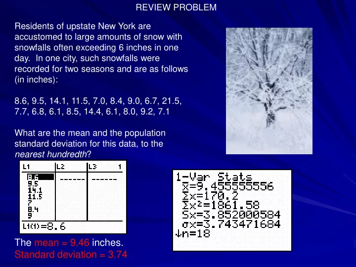
recorded for two seasons and are as follows (in inches): 8.6, 9.5, 14.1, 11.5, 7.0, 8.4, 9.0, 6.7, 21.5, 7.7, 6.8, 6.1, 8.5, 14.4, 6.1, 8.0, 9.2, 7.1 What are the mean and the population standard deviation for this data, to the nearest hundredth?

The mean = 9.46 inches. Standard deviation = 3.74

REVIEW PROBLEM

Density Curves & Normal Distribution

Some Call it a “Bell Curve”

DENSITY CURVES

Density curves give us a mathematical model for distributions. Density curves: are always on or above horizontal axis have an area of exactly 1 underneath it

Centers of Density Curves

MEDIAN—equal-areas point MEAN—balance point The two are equal for a symmetric density curve.

The mean is pulled towards the tail in a skewed curve.

In a skewed curve Median = Equal Areas Mean = Balance Point

NORMAL DISTRIBUTIONS

We use (mu) to represent the mean and (sigma) to represent the standard deviation of a normal distribution.

“Empirical Rule” 68-95-99.7 Rule

Normal Distribution

A normal distribution is a continuous, symmetrical, bell-shaped distribution of a variable.

Characteristics of Normal Distribution

• 1. A normal distribution curve is bell-shaped.
• 2. The mean, median, and mode are equal and

are located at the center of the distribution.

• 3. The curve is unimodal (i.e., it has only one

mode)

• 4. The curve is symmetric about the mean (its

shape is the same on both sides of a vertical line passing through the center)

• 5. The curve is continuous. There are no gaps
• r holes. For each value of X, there is a

corresponding value of Y.

Characteristics of Normal Distribution

• 6. The curve never touches the x axis. No

matter how far in either direction the curve extends, it never meets the x axis – but it gets increasingly closer.

• 7. The total area under a normal distribution

curve is equal to 1.00, or 100%.

The area under the part of a normal curve that lies within 1 standard deviation of the mean is approximately 0.68, or 68%; within 2 standard deviations, about 0.95, or 95%; and within 3 standard deviations, about 0.997, or 99.7%.

The Empirical Rule

(a.k.a. the “68-95-99.7 Rule”)

In a normal distribution, almost all data will lie within 3 standard deviations of the mean.

• About 68% of all data lies within 1 standard

deviation of the mean.

• About 95% of all data lies within 2 standard

deviations of the mean.

• About 99.7% of all data lies within 3 standard

deviations of the mean.

Why Do We Need It?

The Empirical Rule is most often used in statistics for forecasting or predicting final

• utcomes.

After a standard deviation is calculated, and before exact data can be collected, the Empirical Rule can be used to estimate impending data. The probability based on the Empirical Rule can be used if gathering appropriate data may be time consuming, or even impossible to obtain.

Tips for Using the Empirical Rule

Before applying the Empirical Rule it is a good idea to identify the data being described and the value of the mean and standard deviation. Sketch a graph summarizing the information provided by the empirical rule and identify the percentages for each region of the graph (+/- 1, +/- 2, +/- 3) Remember that data must be normally distributed for the Empirical Rule to apply.

The Empirical Rule for a Normal Distribution

STEPS FOR FINDING NORMAL PROPORTION

• 1. State the problem in terms of

x, your variable of concern.

• 2. Standardize the variable.
• 3. Draw a picture & shade area
• f concern.
• 4. Use the table to determine

proportion.

From Proportion to Real Value GOING BACKWARDS!

• 1. State the problem.
• 2. Use the table.
• 3. Draw & shade a picture.
• 4. Unstandardize to obtain your x.

The amount of mustard dispensed from a machine at The Hotdog Emporium is normally distributed with a mean

• f 0.9 ounce and a standard

deviation of 0.1 ounce. If the machine is used 500 times, approximately how many times will it be expected to dispense 1 or more

• unces of mustard.

Choose: 5 16 80 100 The mean is 0.9 and the standard deviation is 0.1. If one standard deviation is added to the mean, the result is 1.0 ounce. Therefore, dispensing 1 or more

• unces falls into the category above one standard deviation to the right of the
• mean. Using the Empirical Rule, 16% of data falls at or above 1 standard

deviation. 16% x 500 = 80 times to dispense one or more ounces of mustard.

A machine is used to fill soda bottles. The amount of soda dispensed into each bottle varies slightly. Suppose the amount of soda dispensed into the bottles is normally distributed. If at least 99% of the bottles must have between 585 and 595 milliliters of soda, find the greatest standard deviation, to the nearest hundredth, that can be allowed. The 99% implies a distribution within 3 standard deviations of the mean. The difference from 585 milliliters to 595 milliliters is 10 milliliters. Symmetrically divided, there are 5 milliliters used to create 3 standard deviations on one side of the mean. Dividing 5 by 3, we get the standard deviation to be 1.67 milliliters, to the nearest hundredth.

Battery lifetime is normally distributed for large

• samples. The mean lifetime is 500 days and

the standard deviation is 61 days. To the nearest percent, what percent of batteries have lifetimes less than 439 days? Subtracting, we see that 1 s.d. below is 439 days, an exact match to

• ur question and an indication that the Empirical Rule can be used to

find the answer. The question is asking what percent of a distribution is beyond one standard deviation to the left of the mean. Answer: 16%

A shoe manufacturer collected data regarding men's shoe sizes and found that the distribution of sizes exactly fits the normal curve. If the mean shoe size is 11 and the standard deviation is 1.5, find:

• a. the probability that a man's shoe size

is greater than or equal to 11.

• b. the probability that a man's shoe size

is greater than or equal to 14.

• a. 50% In a normal distribution, the mean divides the data into two equal
• areas. Since 11 is the mean, 50% of the data is above 11 and 50% is below 11.
• b. 14 is exactly two standard deviations above the mean. Using the Empirical Rule

we see that 2.5% will fall above two standard deviations. Probability is 0.025.

Five hundred values are normally distributed with a mean of 125 and a standard deviation of 10.

• a. What percent of the values lies in the interval 115 - 135,

to the nearest percent?

• b. What interval about the mean includes 95% of the data?
• a. What percent of the values is in the interval 115 - 135?

mean + one standard deviation = 135 mean - one standard deviation = 115 Percent within one standard deviation of the mean = 68%

• b. 2 standard deviations about the mean for a total interval size
• f 40, with the mean in the center.

mean + 2 standard deviations = 145 mean - 2 standard deviations = 105 Interval: [105,145]

Example: Estimating with the Empirical Rule

You have purchased fluorescent light bulbs for your home. The average bulb life is 500 hours with a standard deviation of

• 24. The data is normally distributed.

One of your bulbs burns out at 450 hours. Would you send the bulb back for a refund?

Problem: You have purchased fluorescent light bulbs for your home. The average bulb life is 500 hours with a standard deviation of 24. The data is normally distributed. One of your bulbs burns out at 450 hours. Would you send the bulb back for a refund?

Solution:

According to the Empirical Rule:

• 68% of the light bulbs should last between

500 ± 24 or between 476 to 524 hours.

• 95% of the light bulbs should last between

500 ± 2(24) or between 452 to 548 hours.

• 99.7% of the light bulbs should last between

500 ± 3(24) or between 428 to 572 hours.

If the light bulb only lasted 450 hours, I would consider it a defective bulb. Less than 2.5% should last less than 452 hours.

Your Turn

The scores for all high school seniors taking the verbal section of the Scholastic Aptitude Test (SAT) in a particular year had a mean of 490 and a standard deviation of 100. The distribution of SAT scores is normal.

• 1. What percentage of seniors scored between 390

and 590 on this SAT test?

• 2. One student scored 795 on this test. How did this

student do compared to the rest of the scores?

• 3. A rather exclusive university only admits students

who were among the highest 16% of the scores on this test. What score would a student need on this test to be qualified for admittance to this university?

• 1. What percentage of seniors scored

between 390 and 590 on this SAT test?

The mean = 490 and the standard deviation = 100. So, we can draw the Normal Curve to depict the data.

Calculate the difference between the mean and the test scores: |390-490| = 100  1 s.d. |590-490| = 100  1 s.d. So, about 68% of seniors would score between 390 and 590

• n the SAT test.

• 2. One student scored 795 on this test. How did

this student do compared to the other scores? Calculate the difference between the mean and the

student’s test score:795-390 = 405 This student’s score is more than 3 std. deviations from the mean (3 standard deviations = 3 * 100)

Since about 99.7% of seniors would score between 190 and 790 on the SAT test, this is an exceptionally high score. Only 0.15% of students would have scores above 790. This is an example of using the Empirical Rule to estimate an answer.

3 . A rather exclusive university only admits students who were among the highest 16% of the scores on this

• test. What score would a student need on this test to be

qualified for admittance to this university?

About 68% of the scores are between 390 and 590, so

this leaves 32% of the scores outside this interval. Since a bell-shaped curve is symmetrical, one-half of the scores (16%) are on each end of the distribution.

• 16% of the students scored above 590 on this SAT test.

So, to qualify for admittance to this university, a student would need to score 590 or above on the SAT test.

What if you want to be more precise?

The Empirical Rule works well if we are dealing with values that are exactly 1, 2, or 3 standard deviations away from the mean. It also works well if we simply want to estimate the probability or percentage for a particular value. However, we can be more precise using NORMAL CALCULATIONS which involves standardizing values to obtain z-scores.

STANDARD NORMAL DISTRIBUTION

Standardizing yields z-scores. Use this equation to find the standardized value of x:

x x z

Standard Normal Curve

x has normal distribution of N( , ) z has a standard normal distribution N(0, 1)

The scores for all high school seniors taking the verbal section of the Scholastic Aptitude Test (SAT) in a particular year had a mean of 490 and a standard deviation of 100. The distribution of SAT scores is normal. One student scored 795 on this test. How did this student do compared to the rest of the scores? We estimated before that only 0.15% of students would score above 790, but what percent would score above 795? First, we need to standardize the score of 795. In doing so, we see that this student scored 3.05 standard deviations above the mean of 490.

305 3.05 100

795 490 100 z

The Standard Normal Distribution

Z 0.00 0.01 0.02 0.03 0.04 0.05 0.06 0.07 0.08 0.09 2.0 0.9772 0.9778 0.9783 0.9788 0.9793 0.9798 0.9803 0.9808 0.9812 0.9817 2.1 0.9821 0.9826 0.9830 0.9834 0.9838 0.9842 0.9846 0.9850 0.9854 0.9857 2.2 0.9861 0.9864 0.9868 0.9871 0.9875 0.9878 0.9881 0.9884 0.9887 0.9890 2.3 0.9893 0.9896 0.9898 0.9901 0.9904 0.9906 0.9909 0.9911 0.9913 0.9916 2.4 0.9918 0.9920 0.9922 0.9925 0.9927 0.9929 0.9931 0.9932 0.9934 0.9936 2.5 0.9938 0.9940 0.9941 0.9943 0.9945 0.9946 0.9948 0.9949 0.9951 0.9952 2.6 0.9953 0.9955 0.9956 0.9957 0.9959 0.9960 0.9961 0.9962 0.9963 0.9964 2.7 0.9965 0.9966 0.9967 0.9968 0.9969 0.9970 0.9971 0.9972 0.9973 0.9974 2.8 0.9974 0.9975 0.9976 0.9977 0.9977 0.9978 0.9979 0.9979 0.9980 0.9981 2.9 0.9981 0.9982 0.9982 0.9983 0.9984 0.9984 0.9985 0.9985 0.9986 0.9986 3.0 0.9987 0.9987 0.9987 0.9988 0.9988 0.9989 0.9989 0.9989 0.9990 0.9990

This is part of a standard Normal table that you should be able to read. Since our particular problem deals with a z-score of 3.05, we should go to the last row (3.0) and

• ver to the appropriate column (0.05). We should see that they meet at 0.9989. This is

the proportion TO THE LEFT of our score (of 795). Our question really wants us to consider the proportion to the right. Since the total area under the curve is 1, we can subtract 0.9989 from 1 to yield 0.0011. That means that only 0.11% (compared to estimate of 0.15% from Empirical Rule) of all students scored higher than a 795.

A group of 625 students has a mean age

• f 15.8 years with a standard deviation of

0.6 years. The ages are normally

• distributed. How many students are

younger than 16.2 years? Express answer to the nearest student?

0.4 0.6667 0.6

16.2 15.8 0.6 z

Z 0.00 0.01 0.02 0.03 0.04 0.05 0.06 0.07 0.08 0.09 0.0 0.5000 0.5040 0.5080 0.5120 0.5160 0.5199 0.5239 0.5279 0.5319 0.5359 0.1 0.5398 0.5438 0.5478 0.5517 0.5557 0.5596 0.5636 0.5675 0.5714 0.5753 0.2 0.5793 0.5832 0.5871 0.5910 0.5948 0.5987 0.6026 0.6064 0.6103 0.6141 0.3 0.6179 0.6217 0.6255 0.6293 0.6331 0.6368 0.6406 0.6443 0.6480 0.6517 0.4 0.6554 0.6591 0.6628 0.6664 0.6700 0.6736 0.6772 0.6808 0.6844 0.6879 0.5 0.6915 0.6950 0.6985 0.7019 0.7054 0.7088 0.7123 0.7157 0.7190 0.7224 0.6 0.7257 0.7291 0.7324 0.7357 0.7389 0.7422 0.7454 0.7486 0.7517 0.7549 0.7 0.7580 0.7611 0.7642 0.7673 0.7704 0.7734 0.7764 0.7794 0.7823 0.7852

This z-score yields a percentage less than 16.2 as 74.86%. When we convert that to a number of students we get 466.75 or approximately 467.

Professor Halen has 184 students in his college mathematics lecture class. The scores

• n the midterm exam are normally distributed

with a mean of 72.3 and a standard deviation

• f 8.9. How many students in the class can be

expected to receive a score between 82 and 90? Express answer to the nearest student.

17.7 1.9888 8.9

90 72.3 8.9 z

9.7 1.0899 8.9

82 72.3 8.9 z

Z 0.00 0.01 0.02 0.03 0.04 0.05 0.06 0.07 0.08 0.09 0.9 0.8159 0.8186 0.8212 0.8238 0.8264 0.8289 0.8315 0.8340 0.8365 0.8389 1.0 0.8413 0.8438 0.8461 0.8485 0.8508 0.8531 0.8554 0.8577 0.8599 0.8621 1.1 0.8643 0.8665 0.8686 0.8708 0.8729 0.8749 0.8770 0.8790 0.8810 0.8830 1.2 0.8849 0.8869 0.8888 0.8907 0.8925 0.8944 0.8962 0.8980 0.8997 0.9015 1.3 0.9032 0.9049 0.9066 0.9082 0.9099 0.9115 0.9131 0.9147 0.9162 0.9177 1.4 0.9192 0.9207 0.9222 0.9236 0.9251 0.9265 0.9279 0.9292 0.9306 0.9319 1.5 0.9332 0.9345 0.9357 0.9370 0.9382 0.9394 0.9406 0.9418 0.9429 0.9441 1.6 0.9452 0.9463 0.9474 0.9484 0.9495 0.9505 0.9515 0.9525 0.9535 0.9545 1.7 0.9554 0.9564 0.9573 0.9582 0.9591 0.9599 0.9608 0.9616 0.9625 0.9633 1.8 0.9641 0.9649 0.9656 0.9664 0.9671 0.9678 0.9686 0.9693 0.9699 0.9706 1.9 0.9713 0.9719 0.9726 0.9732 0.9738 0.9744 0.9750 0.9756 0.9761 0.9767

We get 0.9767 and 0.8621 as the probability associated with these 2 z-scores.

Professor Halen has 184 students in his college mathematics lecture

• class. The scores on the midterm exam are normally distributed with a

mean of 72.3 and a standard deviation of 8.9. How many students in the class can be expected to receive a score between 82 and 90? Express answer to the nearest student.

So, we can subtract 0.9767-0.8621 to yield a proportion of 0.1146. This means that 11.46% of all students scored between an 82 and 90. Therefore, roughly 21 (21.0864) of the 184 students scored between an 82 and 90.

We get 0.9767 and 0.8621 as the probability associated with these 2 z-scores.

• 1. Aliens place emphasis on height. For an alien to be a “leader” it would

need to be at least 75 cm tall. What proportion of aliens would qualify?

• 2. Short aliens are often sent to the front lines in battle because they are

smaller targets. All aliens that are under 37 cm tall can expect to be called into duty. What percent of aliens fall into this category?

• 3. What percent of all aliens are between 41 and 71 cm tall?

Aliens have come to visit Earth. We quickly establish that they are shorter than humans. In fact, their heights vary normally with a mean of 50 cm and standard deviation of 10 cm.

• 1. Aliens place emphasis on height. For an alien to be a “leader” it would

need to be at least 75 cm tall. What proportion of aliens would qualify?

Aliens have come to visit Earth. We quickly establish that they are shorter than humans. In fact, their heights vary normally with a mean of 50 cm and standard deviation of 10 cm.

25 2.5 10

75 50 10 z

This yields a proportion of 0.9938 to the left (or 0.0062 to the right).

So, only a proportion

• f 0.0062 of all aliens

would qualify for a leadership positions.

• 2. Short aliens are often sent to the front lines in battle because they are

smaller targets. All aliens that are under 37 cm tall can expect to be called into duty. What percent of aliens fall into this category?

Aliens have come to visit Earth. We quickly establish that they are shorter than humans. In fact, their heights vary normally with a mean of 50 cm and standard deviation of 10 cm.

13 1.3 10

37 50 10 z

This yields a proportion of 0.0968 to the left.

Therefore, 9.68% of all aliens should be expected to serve their duty on the front lines of battle.

• 3. What percent of all aliens are between 41 and 71 cm tall?

21 2.1 10

71 50 10 z

Aliens have come to visit Earth. We quickly establish that they are shorter than humans. In fact, their heights vary normally with a mean of 50 cm and standard deviation of 10 cm.

9 0.9 10

41 50 10 z

This yields proportions to the left of 0.9821 and 0.1841.

So, when we subtract these proportions, we find that the proportion of aliens between 41 and 71 cm tall is 0.7980. In other words, approximately 79.80% of all aliens are between 41 and 71 cm tall.