Densely Connected Networks (DenseNet) Densely Connected Networks - PowerPoint PPT Presentation

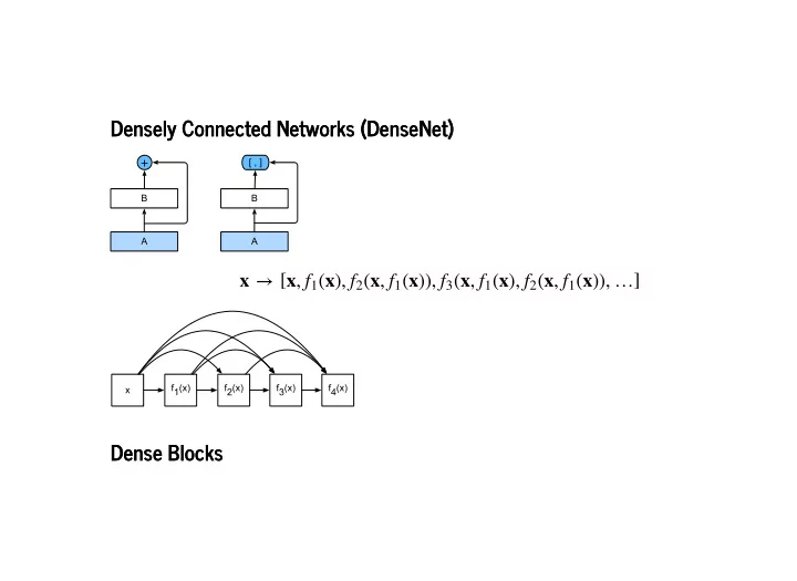
3/8/2019 densenet slides Densely Connected Networks (DenseNet) Densely Connected Networks (DenseNet) x → [ x , ( x )), … ] f 1 ( x ), f 2 ( x , f 1 ( x )), f 3 ( x , f 1 ( x ), f 2 ( x , f 1 Dense Blocks Dense Blocks http://127.0.0.1:8000/densenet.slides.html?print-pdf/#/ 1/8

3/8/2019 densenet slides In [1]: import d2l from mxnet import gluon, init, nd from mxnet.gluon import nn def conv_block(num_channels): blk = nn.Sequential() blk.add(nn.BatchNorm(), nn.Activation('relu'), nn.Conv2D(num_channels, kernel_size=3, padding=1)) return blk http://127.0.0.1:8000/densenet.slides.html?print-pdf/#/ 2/8

3/8/2019 densenet slides A dense block consists of multiple conv_block units, each using the same number of output channels. In the forward computation, however, we concatenate the input and output of each block on the channel dimension. In [2]: class DenseBlock (nn.Block): def __init__(self, num_convs, num_channels, **kwargs): super(DenseBlock, self).__init__(**kwargs) self.net = nn.Sequential() for _ in range(num_convs): self.net.add(conv_block(num_channels)) def forward(self, X): for blk in self.net: Y = blk(X) X = nd.concat(X, Y, dim=1) # Concatenate the input and output of each block on the channel dimension. return X http://127.0.0.1:8000/densenet.slides.html?print-pdf/#/ 3/8

3/8/2019 densenet slides Testing it with data. In [3]: blk = DenseBlock(2, 10) blk.initialize() X = nd.random.uniform(shape=(4, 3, 8, 8)) Y = blk(X) Y.shape (4, 23, 8, 8) Out[3]: http://127.0.0.1:8000/densenet.slides.html?print-pdf/#/ 4/8

3/8/2019 densenet slides Transition Layers to reduce dimensionality Transition Layers to reduce dimensionality In [4]: def transition_block(num_channels): blk = nn.Sequential() blk.add(nn.BatchNorm(), nn.Activation('relu'), nn.Conv2D(num_channels, kernel_size=1), nn.AvgPool2D(pool_size=2, strides=2)) return blk In [5]: blk = transition_block(10) blk.initialize() print(Y.shape) print(blk(Y).shape) (4, 23, 8, 8) (4, 10, 4, 4) http://127.0.0.1:8000/densenet.slides.html?print-pdf/#/ 5/8

3/8/2019 densenet slides DenseNet Model DenseNet Model In [6]: net = nn.Sequential() net.add(nn.Conv2D(64, kernel_size=7, strides=2, padding=3), nn.BatchNorm(), nn.Activation('relu'), nn.MaxPool2D(pool_size=3, strides=2, padding=1)) 4 dense blocks with a transition layer in between. In [7]: num_channels, growth_rate = 64, 32 # Num_channels: the current number of channel s. num_convs_in_dense_blocks = [4, 4, 4, 4] for i, num_convs in enumerate(num_convs_in_dense_blocks): net.add(DenseBlock(num_convs, growth_rate)) # This is the number of output channels in the previous dense block. num_channels += num_convs * growth_rate # A transition layer that haves the number of channels is added between the de nse blocks. if i != len(num_convs_in_dense_blocks) - 1: net.add(transition_block(num_channels // 2)) http://127.0.0.1:8000/densenet.slides.html?print-pdf/#/ 6/8

3/8/2019 densenet slides Last stage Last stage Similar to ResNet, a global pooling layer and fully connected layer are connected at the end to produce the output. In [8]: net.add(nn.BatchNorm(), nn.Activation('relu'), nn.GlobalAvgPool2D(), nn.Dense(10)) http://127.0.0.1:8000/densenet.slides.html?print-pdf/#/ 7/8

3/8/2019 densenet slides Data Acquisition and Training Data Acquisition and Training Since we are using a deeper network here we only use 96x96 images for speed. In [9]: lr, num_epochs, batch_size, ctx = 0.1, 5, 256, d2l.try_gpu() net.initialize(ctx=ctx, init=init.Xavier()) trainer = gluon.Trainer(net.collect_params(), 'sgd', {'learning_rate': lr}) train_iter, test_iter = d2l.load_data_fashion_mnist(batch_size, resize=96) d2l.train_ch5(net, train_iter, test_iter, batch_size, trainer, ctx, num_epochs) training on gpu(0) epoch 1, loss 0.5356, train acc 0.811, test acc 0.866, time 15.0 sec epoch 2, loss 0.3142, train acc 0.886, test acc 0.829, time 13.2 sec epoch 3, loss 0.2647, train acc 0.904, test acc 0.904, time 13.2 sec epoch 4, loss 0.2304, train acc 0.917, test acc 0.909, time 13.2 sec epoch 5, loss 0.2105, train acc 0.923, test acc 0.915, time 13.2 sec http://127.0.0.1:8000/densenet.slides.html?print-pdf/#/ 8/8