Definite Integrals Fundamental Theorem of Calculus Slide 3 / 85 - - PDF document

Slide 1 / 85

Definite Integrals

Slide 2 / 85

Table of Contents

Riemann Sums Trapezoid Rule Accumulation Function Antiderivatives & Definite Integrals Mean Value Theorem & Average Value Fundamental Theorem of Calculus

Slide 3 / 85

Riemann Sums

Return to Table of Contents

Slide 4 / 85

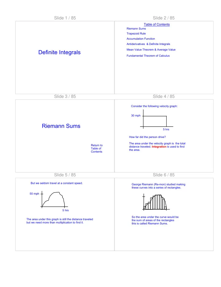
Consider the following velocity graph: 30 mph 5 hrs How far did the person drive? The area under the velocity graph is the total distance traveled. Integration is used to find the area.

Slide 5 / 85

50 mph 5 hrs But we seldom travel at a constant speed. The area under this graph is still the distance traveled but we need more than multiplication to find it.

Slide 6 / 85

George Riemann (Re-mon) studied making these curves into a series of rectangles. So the area under the curve would be the sum of areas of the rectangles this is called Riemann Sums.

Slide 7 / 85

Riemann Sums

Riemann Sums, or Rectangular Approximation Method, is calculated by drawing rectangles from the x-axis up to the curve. The question is: What part of the "top" of the rectangle should lie on the curve? The right hand corner. (RRAM) The left hand corner. (LRAM) The middle. (MRAM)

Slide 8 / 85

Example: Find the area y = x2 and the x-axis [0,1] using Riemann Sums and 4 partitions. 1/4 1/2 3/4 1 Found the width of the rectangle: (b-a)/n= (1-0)/4 LRAM .25f(0) +.25f(.25) +.25f(.5)+.25f(.75) .25(0) + .25(.0625) + .25(.25) + .25(.5625) 0 + .015625 + .0625 + .140625 .21875≈.219 Is this approximation an overestimate or an underestimate?

Slide 9 / 85

Example: Find the area y = x2 and the x-axis [0,1] using Riemann Sums and 4 partitions. 1/4 1/2 3/4 1 Is this approximation an overestimate or an underestimate? RRAM .25f(.25) +.25f(.5)+.25f(.75) + .25f(1) .25(.0625) + .25(.25) + .25(.5625) + .25(1) .015625 + .0625 + .140625 + .25 .46875≈.469

Slide 10 / 85

Example: Find the area y = x2 and the x-axis [0,1] using Riemann Sums and 4 partitions. 1/4 1/2 3/4 1 MRAM .25f(1/8) + .25f(3/8) + .25f(5/8) + .25f(7/8) .25(.015625) + .25(.140625) +.25(.390625) +.25(.765625) .328125≈.328 This value falls between LRAM and RRAM.

Slide 11 / 85

*NOTE: MRAM ≠ LRAM + RRAM 2

There is a downloadable program for finding LRAM, RRAM, & MRAM.

Slide 12 / 85

Q: What units should be used? A: Since the area is found by multiplying base times height, the units of the area are the units of the x-axis times the units of the y-axis. In our example at the beginning of the unit we had a velocity (mph) vs. time (hours) the units would then be

Slide 13 / 85

1 When finding the area between y=3x+2 and the x-axis [1,3] using four partitions, how wide should each interval be?

Slide 14 / 85

2 Find the area between y=3x+2 and the x-axis [1,3] using four partitions and LRAM.

Slide 15 / 85

3 Find the area between y=3x+2 and the x-axis [1,3] using four partitions and RRAM.

Slide 16 / 85

4 When finding the area between y=3x+2 and the x-axis [1,3] using four partitions and MRAM, what in the third rectangle what x should be used in f(x)?

Slide 17 / 85

5 Find the area between y=3x+2 and the x-axis [1,3] using four partitions and MRAM.

Slide 18 / 85

We can write the four areas using where ak is the area of the kth rectangle. It is just another way of writing what we just did. Σ is the Greek letter sigma and stands for the summation of all the terms evaluated at starting with the bottom number and going through to the top.

Slide 19 / 85

Selected Rules for Sigma

Slide 20 / 85

Equivalent Formulas

1st n integers: 1st n squares: 1st n cubes:

Slide 21 / 85

6

55

Slide 22 / 85

7

• 91

Slide 23 / 85

8

1million

Slide 24 / 85

9

• 20

Slide 25 / 85

Trapezoid Rule

Return to Table of Contents

Slide 26 / 85

Example: Find the area y = x2 and the x-axis [0,1] using 4 partitions. 1/4 1/2 3/4 1 Why were areas found using RAM only estimates? How could we draw lines to improve our estimates? What shape do you get?

Slide 27 / 85

Example: Find the area y = x2 and the x-axis [0,1] using 4 partitions and the trapezoids. 1/4 1/2 3/4 1 Trapezoids

Slide 28 / 85 *NOTE: Trapezoid Approximation = LRAM + RRAM 2

We could make our approximation even closer if we used parabolas instead of lines as the tops of our intervals. This is called Simpson's Rule but this is not on the AP Calc AB exam.

Slide 29 / 85

10 The area between y = and the x-axis [1,3] is approximated with 5 partitions and trapezoids. What is the height of each trapezoid?

Slide 30 / 85

11 The area between y = and the x-axis [1,3] is approximated with 5 partitions and trapezoids. What is the area of the 5th trapezoid?

Slide 31 / 85

12 The area between y = and the x-axis [1,3] is approximated with 5 partitions and trapezoids. What is the approximate area?

Slide 32 / 85

13 What is the approximate area using the trapezoids that are drawn?

Slide 33 / 85

14 What is the approximate fuel consumed using the trapezoids rule for this hour flight?

Time (minutes) Rate of Consumption (gal/min) 10 20 25 30 40 40 60 45

Slide 34 / 85

In the last 2 responder questions, the partitioned intervals weren't uniform. The AP will use both. So don't assume.

Slide 35 / 85

So far we have been summing areas using Σ. Gottfried Leibniz, a German mathematician, came up with a symbol you're going to see a lot of: ∫. It is actually the German S instead of the Greek. It still means summation. As a point of interest, we use the German notation in calculus because Leibniz was the first to publish. Sir Isaac Newton is now given the credit for unifying calculus because his notes predate Leibniz's.

Slide 36 / 85

Accumulation Function

Return to Table of Contents

Slide 37 / 85

Another way we can calculate area under a function is to use geometry. V (m/s) t (sec) What's happening during t=0 to t=3? What is the area of t=0 to t=3? What does the area mean? What is the acceleration at t=3? What is happening during t=3 to t=6? What is the area of t=3 to t=6? What does this area mean? Where is the object at t=6 in relation to where it was at t=0?

Slide 38 / 85

The symbol notation for the area from zero to 3: "The area from t=0 to t=3 is the integral from 0 to 3 of the velocity function with respect to t." In general:

Slide 39 / 85

What is the area from x=-4 to x=0? What does this area mean? What is the object's position at x=0 in relation to x=-4? What is the object's position at x=-4 in relation to x=0?

Slide 40 / 85

When solving an accumulation function: (direction)(relation to x-axis)(area)

Slide 41 / 85

15

semicircle

Slide 42 / 85

16

semicircle

Slide 43 / 85

17

semicircle

Slide 44 / 85

18

semicircle

Slide 45 / 85

19

semicircle

Slide 46 / 85

Antiderivatives & Definite Integrals

Return to Table of Contents

Slide 47 / 85

Area under the curve of f(x) from a to b is We have been using geometry to find A. The antiderivative of f(x) can also be used.

Slide 48 / 85

Properties of Definite Integrals

Slide 49 / 85

20

Slide 50 / 85

21

Slide 51 / 85

22

Slide 52 / 85

23

Slide 53 / 85

Antiderivative Rules

Slide 54 / 85

Where F(x) is the anti derivative of f(x).

Slide 55 / 85

Examples: Notice how C always disappears? We don't need when we do definite integrals.

Slide 56 / 85

24

Slide 57 / 85

25

Slide 58 / 85

26

Slide 59 / 85

27

Slide 60 / 85

28

Slide 61 / 85

29

Slide 62 / 85

30

Slide 63 / 85

*Spoiler Alert* *Spoiler Alert* *Spoiler Alert* *Spoiler Alert* You can do definite integrals on your graphing calculator. For the TI-84: use the MATH key 9: fnInt( For example: Depending on which version of the operating system you have:

Slide 64 / 85

The graphing calculator also has a built-in integration function. MATH -> 9:fnInt( depending on the version of the operating system: fnInt( or For example, integrate x2 - 3 from 1 to 4 with respect to x. fnInt(x 2 - 3,x,1,4)

Slide 65 / 85

Mean Value Theorem & Average Value

Return to Table of Contents

Slide 66 / 85

50 mph 5 hrs Think back to this example from the beginning of the unit. The area under this graph is the distance traveled. What is the average rate of speed for this trip? Total distance / total time. How can we use integrals to express this?

Slide 67 / 85

Average Value

Slide 68 / 85

How can this be used? Think Easy Pass on the Parkway or Turnpike. Your time through a booth is recorded and recorded again at the next booth which is a known distance apart. Distance b-a

• ops, ticket in the mail!

Slide 69 / 85

50 mph 5 hrs Using that same graph of our trip, let' say the average speed was 50 mph. This means there are some times where are speed is less than 50 mph and some where it is more than 50 mph. By the Intermediate Value Theorem, There must be at least one time, c, when are speed is exactly 50 mph. This is the Mean Value Theorem

Slide 70 / 85

The Mean Value Theorem

• r

Slide 71 / 85

Ex: Find c that satisfies the Mean Value Theorem for

Slide 72 / 85

Ex: Find c that satisfies the Mean Value Theorem for since -2 is not on [-1,2] c=2/3

Slide 73 / 85

Ex: Find c that satisfies the Mean Value Theorem for

Slide 74 / 85

31 Find c that satisfies the Mean Value Theorem for

Slide 75 / 85

32 Find c that satisfies the Mean Value Theorem for

Slide 76 / 85

33 Find c that satisfies the Mean Value Theorem for

Slide 77 / 85

34 Find c that satisfies the Mean Value Theorem for

Slide 78 / 85

Fundamental Theorem of Calculus

Return to Table of Contents

Slide 79 / 85

There are 2 parts to the Fundamental Theorem of Calculus, depending on the book, the order will change.

Fundamental Theorem of Calculus (F.T.C.)

Part 1 If f(x) is continuous at every point of [a,b] and F(x) is the antiderivative of f(x) then (which is what you've been doing)

Slide 80 / 85

Fundamental Theorem of Calculus (F.T.C.)

Part 2 If F(x) is continuous at every point of [a,b] then has a derivative at every pint on [a,b],and

Slide 81 / 85

Example: It looks easy, but be aware. When the derivative of the bounds in anything other that 1, need to multiply f(x) by the derivative.

Slide 82 / 85

35

A B C D

Slide 83 / 85

36

A B C D

Slide 84 / 85

37

A B C D HINT

Slide 85 / 85

38

A B C D

HINT