Dedicated Computers for (H igh-Energy) Physics R. Tripiccione - PowerPoint PPT Presentation
Dedicated Computers for (H igh-Energy) Physics R. Tripiccione Physics Department, Universita' di Ferrara tripiccione@fe.infn.it Arcetri, September 20th, 2005 Outline of this talk Why dit it happen that quite a few theoretical physicists turned
Dedicated Computers for (H igh-Energy) Physics R. Tripiccione Physics Department, Universita' di Ferrara tripiccione@fe.infn.it Arcetri, September 20th, 2005
Outline of this talk Why dit it happen that quite a few theoretical physicists turned into computer builders? Why was it possible? Three examples: Stellar dynamics (GRAPE) Lattice QCD (mostly APE) Spin-glass systems (SUE/IANUS) Conclusions: What did we learn? Whar are we going to learn next?
The main point of this talk In many cases, computing accurate predictions of the behaviour of a physical system is hopeless, unless numerical techniques are used
The main point of this talk In many cases, computing accurate predictions of the behaviour of a physical system is hopeless, unless numerical techniques are used However Nature has been friendly to us
The main point of this talk In many cases, computing accurate predictions of the behaviour of a physical system is hopeless, unless numerical techniques are used However Nature has been friendly to us so the (simple) physics laws behind the behaviour of computers make it relatively easy to build machine that simulate complex physics!!!!
Some problems are really computationally challenging: Example 1: Stellar dynamics Just try to integrate the equation of motion of N start in gravitational interaction among them N ∀ i, V i = ∑ j j / r ij O N While a time step is 2 O N Computing the forces is What if you have a simple object (a globular cluster ~10 6 bodies)?
Example 2: Lattice Quantum Chromo-Dynamics Unfortunately it is not yet known whether the quarks in Quantum Chromodynamics actually form the required bound states. To establish whether these bound states exist one must solve a strong coupling problem and present methods for solving field theories don't work for strong coupling. K. Wilson, Cargese Lectures, 1976
Example 2: Lattice Quantum Chromo-Dynamics The “obvious” solution is to make the path-integral approach numerically manageable by going to a discrete and finite lattice and using Monte Carlo techniques − S g U ⋅ ∫ D [] e − M [ U ] P U ~ e which boils down to findind the determinant of the sparse but hugely large Dirac op. M M xy U y = xy − H xy U y The lattice spacing has to be small enough that no UV problems are present, HOWEVER The Lattice size has to be much larger than the Compton length of your lightest particle
There have been several attempt at parametrizing phenomenologically the computational s k l complexity of the problem: a t s ' r e h c s u L 6 m . M 5 ⋅ 7 C ∝ ⋅ L / L 0 a 0 / a , m z c i b u L . y V a d o t The experimentally measured values are challenging indeed:
Example 3: Spin Glasses y a d r e t s e y , A very simple Hamiltonian (defined on e.g. a discrete 3-D lattice) k l a t s ' i s H =− ∑ NB ij i J ij j , ={ 1, − 1 } i J ={ 1, − 1 } r a P . G may hide a tremendously complex dynamics, due to the extremely irregular energy landscape in the configuration space Here one may want to study e.g., the phase structure of the model.
Better computers than those you can buy? Fine: you need a lot of computing power, BUT .... ... Why on earth do you think you can do better than an established computer industry? Two answers to this question: 1) What we need is not exactly what traditional computers have been good at AND 2) What we need is very simple to achieve in terms of computer architecture ... ... if we proceed in the direction that basic physics laws point to us
Better computers than those you can buy? 1) What we need is not exactly what traditional computers have been good at Either we need long straight sequences of complex mathematical (f.p.) operations 1 / r 2 e.g.: (stellar dynamics) a × b c or: among complex numbers (LQCD) or conversely, we need long straight sequences of extremely simple boolean operations ∑ NB ij i J ij j
Better computers than those you can buy? 2) What we need is very simple to achieve in terms of computer architectue Basic physics help us in many ways: 1) Parallel computing is trivially possible in all cases ... ... and parallel computing is the physics sponsored way to compute: The basic object is the transistor 0 Industry learns to build smaller and smaller transistors. As 2 N ∝ 1 / ∝ obviously but speed scales more weakly that is: it will increasing convenient to do more and more things in parallel rather than to do a fixed number of things faster and faster
Better computers than those you can buy? 2) What we need is very simple to achieve in terms of computer architectue Basic physics helps us in two ways: 2) We are interested in modeling local theories: This goes (must go) over to the computer structure -> Keep data close in space to where it is processed Failure to do so will asymptotically bring a data bottleneck: 2 P L ∝ L B L ∝ L does not work in stellar dynamics, but there B ≃ P
An historical remark: Doing things one after the other (serially) Keeping data storage and data processing separated (in principle and practice) are the cornerstones of the famous von Neumann model of computing Q: So was Von Neumann wrong? P 0 A: No, simply he was interested in the regime P ∞ while today we are approaching the regime .....
Better computers than those you can buy? These advantages have been exploited in big projects and small projects: Stellar dynamics and LQCD are examples of big projects Spin Glass simulation engines are much more back yard attempts.
Important dates in LQCD computing 1979: The early pioneers: the Caltech Ising machine (D. Toussant, G. Fox, C. Seitz) circa 1985: APE (16 nodes, 1 Gflops) Columbia (~ 1 Gflops) GF11 (IBM/Yorktown) 1990 - 1995: APE100 (500 – 1000 nodes, 50 – 100 Gflops) Columbia2 (also about 100 Gflops) 1995 – 2000: APEmille (1.8 Tflops installed) QCDSP (1 + 1 Tflops at Columbia & Broohhaven) CP-PACS (Tsukuba + Hitachi, 600 Gflops) 2000 – 2005: apeNEXT QCDOC (Columbia + Brookhaven + IBM/Yorktown)
The apeNEXT structure The apeNEXT structure is a 3-D grid of processing elements each holding its fair share of memory Each processor does at its best what (and only what) is needed for LQCD
APE gallery “It is easy! It may as well turn out to be possible.....” G. Parisi, Spring 1985
ApeNEXT picture Gallery
A less obvious example: numerical relativity In numerical relativity things are less stable ---> better to use (at best) traditional machines University Network AlbertNEXT Gigabit Ethernet Switch 1000x24 Switch 1000x24 Infiniband 24 port switch Albert016 Albert015 Albert014 L. Baiotti, et al,, Phys.Rev.Lett.94:131101,2005 Albert003 A. Nagar etal., Phys.Rev.D72:024007,2005 Albert002 Albert001
GRAPE GRAPE concentrates on computing the potential, the force, and its derivative. It has been consistently the fastest computer on Earth ~ 70 Tflops equivalent (with some reasonable normalization factor) Eacj element of the machine computes forces for N/P stars bl
SUE Monte Carlo simulation of an //---------------------------------------- Ising spin glass is just a few lines void update(J) H =− ∑ NB ij i J ij j double J; of C code { int i, j, tp; double deltaE, rndValue; double prob; SUE perform the complete for(i=1; i<=SIZE; i++) { for(j=1; j<=SIZE; j++) { computation in hardware deltaE = (double)(2*spin[i][j]*(spin[i+1][j]+spin[i-1][j]+spin[i][j+1]+spin[i] [j-1])); deltaE = J * deltaE; At the same time on many replicas if(e deltaE < 0.0) spin[i][j] = -spin[i][j]; else { rndValue = (double) random() / ((double) RAND_MAX) ; spin[i][j] = rndValue < exp(-deltaE) ? -spin[i][j] : spin[i][j]; The original machine (~1998) } updates on average one spin in } // end of for_j } // end of for_i ~ 200 ps }
SUE Typical physics result: make sure you have brought to equilibrium a 203 lattice, and explore its phase structure (Ballesteros et al., cond-mat/0006211 At the age of 7, SUE is roughly equivalent to a small-size high-end PC cluster (say 32 PC's) + state-of-the-art program writing however ....
superSUE / IANUS A new scaled up version, to be ready in summer next year, will improve by a factor ~ 500, breaking the 1 ps / spin-update barrier that is ~ 10000 PC's working all together on the same problem... at the cost of ~ 300 PC's preliminary tests already available ------>
Conclusions Quite often traditional computers do not do exaclty what physics simulation needs most And more often than not they do it the “wrong way” (from the physics point of view) This provides an opportunity for physicists to build their own computing tools Recent developments seem to signal that industry is slowly learning that it is better to follow physics than fighting against it (IBM Blue Gene/L) so we may hope that computers for physics will be readily available soon ... “... and I' ll be able to do something else at last”
Recommend
More recommend
Explore More Topics
Stay informed with curated content and fresh updates.
