
Dataflow analysis
Michel Schinz Advanced compiler construction, 2008-05-09
First example (analysis #1) Available expressions
Common subexp. elimination
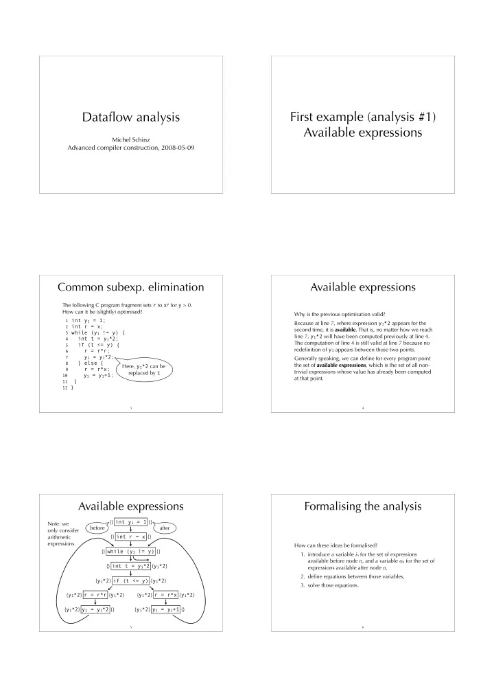
The following C program fragment sets r to xy for y > 0. How can it be (slightly) optimised? 1 int y1 = 1; 2 int r = x; 3 while (y1 != y) { 4 int t = y1*2; 5 if (t <= y) { 6 r = r*r; 7 y1 = y1*2; 8 } else { 9 r = r*x;
10 y1 = y1+1; 11 } 12 }
3
Here, y1*2 can be replaced by t
Available expressions
Why is the previous optimisation valid? Because at line 7, where expression y1*2 appears for the second time, it is available. That is, no matter how we reach line 7, y1*2 will have been computed previously at line 4. The computation of line 4 is still valid at line 7 because no redefinition of y1 appears between those two points. Generally speaking, we can define for every program point the set of available expressions, which is the set of all non- trivial expressions whose value has already been computed at that point.
4
Available expressions
5
int y1 = 1 int r = x while (y1 != y) int t = y1*2 if (t <= y) r = r*r y1 = y1*2 r = r*x y1 = y1+1 {} {} {} {} {} {} {} {y1*2} {y1*2} {y1*2} {y1*2} {y1*2} {y1*2} {} {y1*2} {} {y1*2} {y1*2} before after Note: we
- nly consider
arithmetic expressions.
Formalising the analysis
6
How can these ideas be formalised?
- 1. introduce a variable in for the set of expressions
available before node n, and a variable on for the set of expressions available after node n,
- 2. define equations between those variables,
- 3. solve those equations.