
Data Preparation
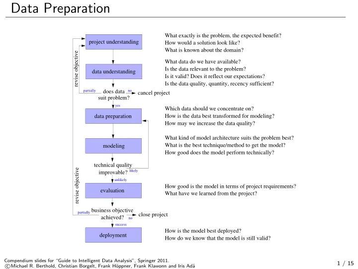
project understanding cancel project revise objective technical quality improvable? business objective achieved? revise objective close project suit problem? does data
no success partially partially no yes
How would a solution look like? What is known about the domain? What exactly is the problem, the expected benefit? What data do we have available? Is the data relevant to the problem? Is it valid? Does it reflect our expectations? Is the data quality, quantity, recency sufficient? Which data should we concentrate on? How is the data best transformed for modeling? How may we increase the data quality? What kind of model architecture suits the problem best? What is the best technique/method to get the model? How good does the model perform technically?
likely unlikely
How good is the model in terms of project requirements? What have we learned from the project? How is the model best deployed? How do we know that the model is still valid? data understanding modeling data preparation evaluation deployment
Compendium slides for “Guide to Intelligent Data Analysis”, Springer 2011. c Michael R. Berthold, Christian Borgelt, Frank H¨
- ppner, Frank Klawonn and Iris Ad¨
a
1 / 15