
SLIDE 1
Darcy’s Law into Continuity Equation
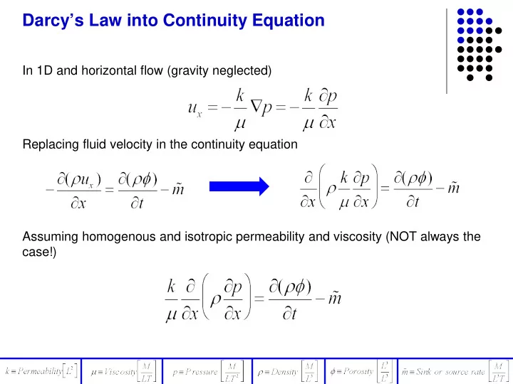
In 1D and horizontal flow (gravity neglected) Replacing fluid velocity in the continuity equation Assuming homogenous and isotropic permeability and viscosity (NOT always the case!)
Darcys Law into Continuity Equation In 1D and horizontal flow - - PowerPoint PPT Presentation
Darcys Law into Continuity Equation In 1D and horizontal flow (gravity neglected) Replacing fluid velocity in the continuity equation Assuming homogenous and isotropic permeability and viscosity (NOT always the case!) Formation Volume Factor
In 1D and horizontal flow (gravity neglected) Replacing fluid velocity in the continuity equation Assuming homogenous and isotropic permeability and viscosity (NOT always the case!)
We measure volume at surface but do the mass balance at the reservoir
SC RC w
Formation volume factor and ρ depend on both pressure and temperature
depth
Surface/Standard Conditions Reservoir Conditions
sc
R R R
At reservoir conditions, density is: Replacing density in continuity equation and divide through by ρSC (a constant) Using the product rule on the left-hand side of the equation
w w sc
2 2
w w w sc
2 2 2
w w w sc
…And chain rule on the left hand side,
A few definitions:
1 1 (rock compressibility) 1 1 1 1 (fluid compressibility) (total compressibility)
P r P w f w w w T T t r f
V c V p p B V c B V p p p B B p c c c φ φ ρ ρ ∂ ∂ = = ∂ ∂ ∂ ∂ ∂ ∂ − = − = = = ∂ ∂ ∂ ∂ = +
2 2 2
w w w w sc
2 2 2
1 1 1 1 1
r f f
w w w w w w w sc c c c
k p P p m B B B x B p B x B p B p t φ φ µ φ ρ ∂ ∂ ∂ ∂ ∂ ∂ + = + − ∂ ∂ ∂ ∂ ∂ ∂ Chain and product rule on time derivative (right hand side) With some manipulation:
2
fluid compressibility
f
LT c M ≡
2
rock compressibility
r
LT c M ≡
Diffusivity constant Mobility Source
t w SC SC
k c k B m q α µφ λ µ ρ ≡ = ≡ = ≡ =
2 2 2
f t w w w sc
≈0 slightly compressible fluid
If the fluid is “slightly compressible” (liquid), the compressibility is small (< 10-5) and constant and terms involving can be ignored. 1D diffusivity (with homogenous fluid and reservoir properties) can be written: If no sources or sinks (wells) are present, we get the “heat equation”
2 2
In 2D (x-y plane) In 3D and potential Φ accounting for gravity
w f w w w T T
p f p c dp
ρ ρ
V1 V2 More Pressure P1 P2
Recall fluid compressibility factor (cf) at constant temperature Integrating from a reference point (p0, ρ0), to any other point
2 3
1 1 ( ) ( ) ( ) ( ) "'( ) ... 2! 3! f x x f x f x x f x x f x x ′ ′′ + ∆ = + ∆ + ∆ + ∆ +
2 3
( )
f
c p p f f
−
2 2 3 3
f f f
f w
Using Taylor series to expand density around a reference density, Differentiate exponential equation for density: For slightly compressible (cf < 10-5 psi-1) liquids, higher order terms are small:
f
Negligible for small cf
Therefore,
Bw
0=1 (assume reference is
standard conditions)
2 2 1 2
init B B
2 2
(2 1) 4 1
n
n t n init L B n
α π
+ ∞ =
Analytical Solution to PDE “Heat” Equation
x=0 x=L
PB1 PB2
p=pinit
Steady state solution Time increasing
2 2
(2 1) 4 1
n
n t n init L B n
α π
+ ∞ =
That was the easy solution… Real reservoirs have:
(and this is just for single phase flow…)
t SC w w
So how do we solve this complex, nonhomogeneous, 3D PDE?
properties
1 2 1 1 2 3 2 2 3 4 3 1
3 2 2
N N N
TP TP Q TP TP TP Q TP TP TP Q TP TP Q
−
− = − + − = − + − = − + =
1 1 n n
P P t t
+ +
+ = + ∆ ∆ B B T Q