Curves and Surfaces CMSC 635 January 15, 2013 - PDF document

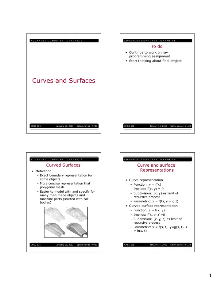
A D V A N C E D C O M P U T E R G R A P H I C S A D V A N C E D C O M P U T E R G R A P H I C S To do • Continue to work on ray programming assignment • Start thinking about final project Curves and Surfaces CMSC 635 January 15, 2013 Spline curves ‹#›/23 CMSC 635 January 15, 2013 Spline curves ‹#›/23 A D V A N C E D C O M P U T E R G R A P H I C S A D V A N C E D C O M P U T E R G R A P H I C S Curved Surfaces Curve and surface Representations • Motivation – Exact boundary representation for some objects • Curve representation – More concise representation that – Function: y = f(x) polygonal mesh – Implicit: f(x, y) = 0 – Easier to model with and specify for – Subdivision: (x, y) as limit of many man-made objects and recursive process machine parts (started with car – Parametric: x = f(t), y = g(t) bodies) • Curved surface representation – Function: z = f(x, y) – Implicit: f(x, y, z)=0 – Subdivision: (x, y, z) as limit of recursive process – Parametric: x = f(s, t), y=g(s, t), z = h(s, t) CMSC 635 January 15, 2013 Spline curves ‹#›/23 CMSC 635 January 15, 2013 Spline curves ‹#›/23 1

A D V A N C E D C O M P U T E R G R A P H I C S A D V A N C E D C O M P U T E R G R A P H I C S Parametric Surfaces Parametric Representation • Boundary defined by parametic • One function vs. many (defined function piecewise) – x = f(u, v) • Continuity – y = f(u, v) • A parametric polynomial curve of order n: – Z = f(u, v) • Example (sphere): – X = sin ( θ ) cos ( φ ) – Y = sin ( θ ) sin ( φ ) – Z = cos( θ ) • Advantages of polynomial curves – Easy to compute – Infinitely differentiable everywhere CMSC 635 January 15, 2013 Spline curves ‹#›/23 CMSC 635 January 15, 2013 Spline curves ‹#›/23 A D V A N C E D C O M P U T E R G R A P H I C S A D V A N C E D C O M P U T E R G R A P H I C S Spline Constructions Bezier Curve • Cubic spline is the most common • Motivation: Draw a smooth intuitive form curve (or surface) given a few key user-specified control points • Common constructions Control point – Bezier: 4 control points – B-splines: approximating C 2 , local control – Hermite: 2 points, 2 normals – Natural splines: interpolating, C 2 , Smooth Bezier curve no local control (drawn automatically) – Catmull-Rom: interpolating, C 1 , local control • Properties: – Interpolates is tangent to end points – Curve within convex hull of control polygon CMSC 635 January 15, 2013 Spline curves ‹#›/23 CMSC 635 January 15, 2013 Spline curves ‹#›/23 2

A D V A N C E D C O M P U T E R G R A P H I C S A D V A N C E D C O M P U T E R G R A P H I C S Linear Bezier Curve deCastljau: Quadratic Bezier Curve • Just a simple linear combination or interpolation (easy to code up, very numerically stable) Quadratic P1 Degree 2, Order 3 F(0) = P0, F(1) = P2 P1 F(1) F(u) = ? P2 Linear (Degree 1, Order 2) P0 F(0) = P0, F(1) = P1 F(u) F(u) = ? P0 P0 P1 P2 F(0) P0 P1 u u 1-u 1-u 1-u u 1-u u F(u) = (1-u) 2 P0 + 2u(1-u) P1 + u 2 P2 F(u) = (1-u) P0 + u P1 CMSC 635 January 15, 2013 Spline curves ‹#›/23 CMSC 635 January 15, 2013 Spline curves ‹#›/23 A D V A N C E D C O M P U T E R G R A P H I C S A D V A N C E D C O M P U T E R G R A P H I C S Geometric Interpretation: Geometric Interpolation: Cubic Quadratic u u u u 1-u 1-u u u u u u CMSC 635 January 15, 2013 Spline curves ‹#›/23 CMSC 635 January 15, 2013 Spline curves ‹#›/23 3

A D V A N C E D C O M P U T E R G R A P H I C S A D V A N C E D C O M P U T E R G R A P H I C S Summary: deCasteljau Summary: deCasteljau Algorithm Algorithm • A recursive implementation of curves • A recursive implementation of curves at different orders at different orders • Further consideration: polar P1 coordinates P1 P2 P1 P2 P0 P3 P0 Quadratic P0 Cubic Degree 2, Order 3 Degree 3, Order 4 Linear F(0) = P0, F(1) = P2 F(0) = P0, F(1) = P3 Degree 1, Order 2 F(0) = P0, F(1) = P1 P0 P1 P2 P0 P1 P2 P3 P0 P1 1-u u 1-u u 1-u u 1-u u 1-u u 1-u u 1-u u 1-u u 1-u u F(u) = (1-u) P0 + u P1 F(u) = (1-u) 2 P0 + 2u(1-u) P1 + u 2 P2 u 1-u F(u) = (1-u) 3 P0 +3u(1-u) 2 P1 +3u 2 (1-u) P2 + u 3 P3 CMSC 635 January 15, 2013 Spline curves ‹#›/23 CMSC 635 January 15, 2013 Spline curves ‹#›/23 A D V A N C E D C O M P U T E R G R A P H I C S A D V A N C E D C O M P U T E R G R A P H I C S Bezier: disadvantages Piecewise polynomial curves • Single piece, no local control (move • Ideas: a control point, whole curve – Use different polynomial functions changes) for different parts of the curve • Complex shapes: can be very high • Advantage: degree, difficult to deal with – Flexibility • In practice: combine many Bezier – Local control curve segments • Issue – But only position continuous at the – Smoothness at joints (G: geometry joint points since Bezier curves continuity: C: derivative continuity) interpolate end-points (which match at segment boundaries) – Unpleasant derivative (slope) discontinuities at end-points CMSC 635 January 15, 2013 Spline curves ‹#›/23 CMSC 635 January 15, 2013 Spline curves ‹#›/23 4

A D V A N C E D C O M P U T E R G R A P H I C S A D V A N C E D C O M P U T E R G R A P H I C S Continuity Continuity • Continuity C k indicates adjacent curves have the same kth derivative • C 1 continuity: Adjacent curves share at their joints – Same endpoints: Q i (1) = Q i+1 (0) and – Same derivative:Q i’ (1) = Q i+1’ (0) • C 0 continuity: Adjacent curves share • C 2 continuity: – Same endpoints: Q i (1) = Q i+1 (0) – Must have C 1 continuity, and – Same second derivatives: Q i ’’(1) = Q i+1 ’’(0) • Most engineering applications (e.g., those in car and airplane industry) require at least C 1 continuity • C -1: discontinuous curves CMSC 635 January 15, 2013 Spline curves ‹#›/23 CMSC 635 January 15, 2013 Spline curves ‹#›/23 A D V A N C E D C O M P U T E R G R A P H I C S A D V A N C E D C O M P U T E R G R A P H I C S Splines A Simple Animation Example • Problem: create a car • More useful form of representation compared to the Bezier curve animation that is driving up • How they work: Parametric curves governed by along the y-axis with control points velocity [0, 3], and arrive at • Mathematically: Several representations to choose the point (0, 4) at time t=0. from. More complicated than vertex lists. See chapter Animate its motion as it 22 of the book for more information. Simple parametric representation: turns and slows down so that at time t=1, it is at position (2, 5) with velocity [2, 0]. • Solution – First step: generate a mathematical • Advantage: Smooth with just a few control point • Disadvantage: Can be hard to control description. • Uses: – Second step: choose the curve – representation of smooth shapes. Either as representation outlines in 2D or with Patches or Subdivision Surfaces in 3D • Hermite curve: r(t)= GMT (t) – animation Paths – approximation of truncated Gaussian Filters • Exercise: Bezier curve representation? CMSC 635 January 15, 2013 Spline curves ‹#›/23 CMSC 635 January 15, 2013 Spline curves ‹#›/23 5

A D V A N C E D C O M P U T E R G R A P H I C S A D V A N C E D C O M P U T E R G R A P H I C S Catmull Rom Spline Subdivision curves • Can be used to solve the following • A simple idea problem. – Using the midpoint of the edge from one point to the next, replace that point with a new one to create a new polygon to construct a new curve. – problem with this? • Further readings: • Solution: – Laplacian interpolation and – Math representation smoothing (Gabriel Taubin @ – Curve construction Brown) • Catmull Rom spline to construct the – Joe Warren@ Rice (on mesh) vectors from the two or three neighbors take home exercise: read chap 22 in the book and construct the curve and the B-spline using the Chen code. CMSC 635 January 15, 2013 Spline curves ‹#›/23 CMSC 635 January 15, 2013 Spline curves ‹#›/23 A D V A N C E D C O M P U T E R G R A P H I C S Surfaces • Curves -> Surfaces • Bezier patch: – 16 points – Check out the Chen code for surface construction CMSC 635 January 15, 2013 Spline curves ‹#›/23 6