Current through a very small conductor nano HUB .org online - - PowerPoint PPT Presentation

nanoHUB.org

Supriyo Datta

1

• nline simulations and more

Network for Computational Nanotechnology

CQT Lecture #4

Unified Model for Quantum Transport Far from Equilibrium

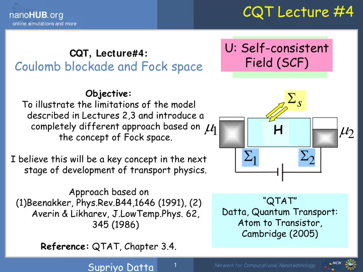
CQT, Lecture#4:

Coulomb blockade and Fock space

Objective: To illustrate the limitations of the model described in Lectures 2,3 and introduce a completely different approach based on the concept of Fock space. I believe this will be a key concept in the next stage of development of transport physics. Approach based on (1)Beenakker, Phys.Rev.B44,1646 (1991), (2) Averin & Likharev, J.LowTemp.Phys. 62, 345 (1986) Reference: QTAT, Chapter 3.4. “QTAT” Datta, Quantum Transport: Atom to Transistor, Cambridge (2005)

U: Self-consistent Field (SCF) H

Σ1

Σ2

μ1 μ2

Σs

nanoHUB.org

Supriyo Datta

2

• nline simulations and more

Network for Computational Nanotechnology

Current through a very small conductor

I = q

• γ1γ2

γ1 + γ2 f1 − f2

[ ]

F = γ1 f1 + γ2 f2 γ1 + γ2 ⎡ ⎣ ⎢ ⎤ ⎦ ⎥

• /

1

γ

γ2 /

μ

1

μ2

• /

1

γ

γ2 /

μ

1

μ2

• 0.2

0.2 0.4 0.6 0.1 0.2 0.3 0.4 0.5 0.6 0.7 0.8 0.9 1

Normalized Current

− qVD ⇒

max I = q

• γ1γ2

γ1 + γ2 ⇒ qγ1 2 if γ2 = γ1 ⇒ qγ1 2

• /

1

γ

γ2 /

μ

1

μ2

• /

1

γ

γ2 /

μ

1

μ2

F

1

f

nanoHUB.org

Supriyo Datta

3

• nline simulations and more

Network for Computational Nanotechnology

Conductance of a very small conductor

• /

1

γ

γ2 /

μ1

μ2

• /

1

γ

γ2 /

μ1

μ2

Normalized Current

Assume γ2 = γ1

• 0.2

0.2 0.4 0.6 0.8

• 0.2

0.2 0.4 0.6 0.8 1

⇒ qγ1 2 T kB 4

− qVD ⇒

Conduc tance = ∂I ∂VD ~ qγ1 /2 2γ1 + 4kBT ~ q2 /4 if γ1 >> kBT

Conduc tance quantum ~ q2 /2π

• /

1

γ

γ2 /

μ

1

μ2

+

1

2γ

nanoHUB.org

Supriyo Datta

4

• nline simulations and more

Network for Computational Nanotechnology

Effect of “U” on conductance

VG VD

CHANNEL D S

I

• /

1

γ

γ2 /

μ1

μ2

• /

1

γ

γ2 /

μ

1

μ2

Normalized Current

• 0.2

0.2 0.4 0.6 0.1 0.2 0.3 0.4 0.5 0.6 0.7 0.8 0.9 1

− qVD ⇒

⇒ qγ1 2 U0 /2

Assume U0 >> kBT , γ1 , γ2

Level floats up by U0 γ2 γ1 + γ2

U0 : Increase in potential due to SINGLE electron Assume γ2 = γ1 U0 = 0.5 eV

nanoHUB.org

Supriyo Datta

5

• nline simulations and more

Network for Computational Nanotechnology

SCF with self-interaction correction

VG VD

CHANNEL D S

I

• /

1

γ

γ2 /

μ1

μ2

• /

1

γ

γ2 /

μ

1

Normalized Current

• 0.2

0.2 0.4 0.6 0.1 0.2 0.3 0.4 0.5 0.6 0.7 0.8 0.9 1

− qVD ⇒

⇒ qγ1 2 U0 /2

Level does NOT float up

Assume γ2 = γ1 U0 = 0.5 eV

Ui = U0 (N − Ni) Self-interaction Correction

nanoHUB.org

Supriyo Datta

6

• nline simulations and more

Network for Computational Nanotechnology

• 0.2

0.2 0.4 0.6 0.8 0.1 0.2 0.3 0.4 0.5 0.6 0.7 0.8 0.9 1

2 levels: Unrestricted SCF

• /

1

γ

γ2 /

μ1

μ2

• /

1

γ

γ2 /

μ1

μ2

Ui = U0 (N − Ni) Self-interaction Correction Ui = U0 N Restricted SCF Unrestricted SCF

• /

1

γ

γ2 /

μ1

μ2

nanoHUB.org

Supriyo Datta

7

• nline simulations and more

Network for Computational Nanotechnology

• 0.2

0.2 0.4 0.6 0.8 0.1 0.2 0.3 0.4 0.5 0.6 0.7 0.8 0.9 1

2 levels: SCF versus exact

• /

1

γ

γ2 /

μ1

μ2

• /

1

γ

γ2 /

μ1

μ2

• /

1

γ

γ2 /

μ1

μ2

Exact Needs picture in “Fock” space One-electron energy levels

nanoHUB.org

Supriyo Datta

8

• nline simulations and more

Network for Computational Nanotechnology

1-level: the view from “Fock space” One-electron picture “Fock space” Most of our thinking is based on this picture

E = ε1

1

E = ε1 E = 0

nanoHUB.org

Supriyo Datta

9

• nline simulations and more

Network for Computational Nanotechnology

2 levels: the view from “Fock space” 2 one-electron levels 2^2 many-electron levels 00 11 01 10

E = 0

E = ε1 E = ε2

E = ε1 + ε2 + U0

E = ε1 E = ε2

nanoHUB.org

Supriyo Datta

10

• nline simulations and more

Network for Computational Nanotechnology

1-level: Current flow in “Fock space”

• /

1

γ

γ2 /

μ1

μ2

• /

1

γ

γ2 /

μ1

μ2

P0 =1

P

1 = 0

P0 = γ1 /(γ1 + γ2)

P

1 = γ2 /(γ1 + γ2)

1

γ2 /

• /

1

γ

1

γ2 /

• /

1

γ

I = (q/) γ1 P

1

= (q/) γ2 P0

• 0.2

0.2 0.4 0.6 0.1 0.2 0.3 0.4 0.5 0.6 0.7 0.8 0.9 1

E = ε1 E = 0 E = ε1 E = 0 ε1 ε1

I = q

• γ1γ2

γ1 + γ2

nanoHUB.org

Supriyo Datta

11

• nline simulations and more

Network for Computational Nanotechnology

2 levels: Current flow in “Fock space”

• 0.2

0.2 0.4 0.6 0.8 0.1 0.2 0.3 0.4 0.5 0.6 0.7 0.8 0.9 1

00 11 01 10

μ1

μ2

• /

1

γ

γ2 /

μ1

μ2

• /

1

γ

γ2 /

μ1

μ2

• /

1

γ

γ2 /

00 11 01 10 00 11 01 10

nanoHUB.org

Supriyo Datta

12

• nline simulations and more

Network for Computational Nanotechnology

2 levels: Current flow in “Fock space”

• 0.2

0.2 0.4 0.6 0.8 0.1 0.2 0.3 0.4 0.5 0.6 0.7 0.8 0.9 1

00 01 10

P

1 = 2γ2 /(γ1 + 2γ2)

P0 = γ1 /(γ1 + 2γ2) I = q

• 2γ1γ2

γ1 + 2γ2 → (2/3) (qγ1 /) I = q

• 2γ1γ2

γ1 + γ2 → (qγ1 /)

I = (q/) γ1 P

1

= (q/) 2γ2 P0

μ1

μ2

• /

1

γ

γ2 /

nanoHUB.org

Supriyo Datta

13

• nline simulations and more

Network for Computational Nanotechnology

Coulomb blockade and strong correlation 00 11 01 10

μ

1 μ2

• /

1

γ

γ2 /

P

00 =(1− f↑)*(1− f↓)

P

10 = f↑*(1− f↓)

P

01 =(1− f↑)* f↓

P

11 = f↑* f↓

• 0.2

0.2 0.4 0.6 0.8 0.1 0.2 0.3 0.4 0.5 0.6 0.7 0.8 0.9 1

P00 = γ1 /(γ1 + 2γ2) P

10 = P01 = γ2 /(γ1 + 2γ2)

P

11 = 0

STRONGLY CORRELATED “UNCORRELATED”

↑

f

↓

f

and

nanoHUB.org

Supriyo Datta

14

• nline simulations and more

Network for Computational Nanotechnology

• 0.5

0.5 1 1.5 2 0.1 0.2 0.3 0.4 0.5 0.6 0.7 0.8 0.9 1

4 levels: USCF versus exact

μ1

μ2

• /

1

γ

γ2 /

Unrestricted SCF

Exact Fock space approach

USCF plateaus have wrong width: U0/2 wrong height: 1/N

N U Ui =

Restricted SCF

Ui = U0 (N − Ni)

nanoHUB.org

Supriyo Datta

15

• nline simulations and more

Network for Computational Nanotechnology

Equilibrium is different …

• 0.5

0.5 1 1.5 2 0.1 0.2 0.3 0.4 0.5 0.6 0.7 0.8 0.9 1

• 0.5

0.5 1 1.5 2 0.5 1 1.5 2 2.5 3 3.5 4

μ1

μ2

• /

1

γ

γ2 /

Normalized Current

− qVD ⇒ μ1 = μ2 ⇒

Number

• f electrons

Non-equilibrium Equilibrium

Exact

SCF: Restricted and unrestricted

nanoHUB.org

Supriyo Datta

16

• nline simulations and more

Network for Computational Nanotechnology

Being “close” to equilibrium helps too

• 0.5

0.5 1 1.5 2 0.1 0.2 0.3 0.4 0.5 0.6 0.7 0.8 0.9 1

μ1

μ2

• /

1

γ

γ2 /

Normalized Current

− qVD ⇒

• --> Closer ---> to equilibrium --->

Exact

SCF: Restricted and unrestricted

γ2 = 100 γ1 γ2 = γ1

• 0.5

0.5 1 1.5 2 0.2 0.4 0.6 0.8 1

• 0.5

0.5 1 1.5 2 0.2 0.4 0.6 0.8 1

γ2 = 10 γ1

nanoHUB.org

Supriyo Datta

17

• nline simulations and more

Network for Computational Nanotechnology

General “Fock space” approach

2 one-electron levels

2^2 many-electron levels

• /

1

γ

γ2 /

μ1

μ2

ε

ε+U0

00 11 01 10

E =0

E =2ε+U0

E =ε

γ1 (1− f1(ε)) γ1 f1(ε) γ1 (1− f1(ε +U0)) γ1 f1(ε+U0)

nanoHUB.org

Supriyo Datta

18

• nline simulations and more

Network for Computational Nanotechnology

Equilibrium in “Fock space”

• /

1

γ

γ2 /

μ1

μ2

ε ε+U0

00 11 01 10

E=0

E=2ε+U0

E =ε

γ1 (1− f1(ε)) γ1 (1− f1(ε+U0)) γ1 f1(ε) γ1 f1(ε+U0)

P

i =

1 Z e− (Ei−μNi) /kBT

PN+1 PN = ⇑ ⇓ = f1(ΔE) 1− f1(ΔE) = e− (ΔE−μ) /kBT

No general solution

• ut-of-equilibrium with µ2 ≠ µ1

Law of Equilibrium

nanoHUB.org

Supriyo Datta

19

• nline simulations and more

Network for Computational Nanotechnology

Rate equations in “Fock space” 00 11 10 01

E =0

E =2ε+U0

E =ε γ1 f

1(ε)

+γ2 f

2(ε)

γ1 f1(ε) +γ2 f2(ε) γ1 f

1(ε+U0)

+γ2 f

2(ε+U0)

γ1 f1(ε+U0) +γ2 f2(ε+U0)

0 0 0 0

Each column adds to zero

d dt P00 P01 P10 P11 ⎧ ⎨ ⎪ ⎪ ⎩ ⎪ ⎪ ⎫ ⎬ ⎪ ⎪ ⎭ ⎪ ⎪ = ⎧ ⎨ ⎪ ⎪ ⎩ ⎪ ⎪ ⎫ ⎬ ⎪ ⎪ ⎭ ⎪ ⎪ = ∗ ∗ ∗ ∗ ⎡ ⎣ ⎢ ⎢ ⎢ ⎢ ⎤ ⎦ ⎥ ⎥ ⎥ ⎥ P00 P01 P10 P11 ⎧ ⎨ ⎪ ⎪ ⎩ ⎪ ⎪ ⎫ ⎬ ⎪ ⎪ ⎭ ⎪ ⎪

nanoHUB.org

Supriyo Datta

20

• nline simulations and more

Network for Computational Nanotechnology

Solving the rate equations 00 11 01 10

E =0

E =2ε+U0

E =ε

1 ⎧ ⎨ ⎪ ⎪ ⎩ ⎪ ⎪ ⎫ ⎬ ⎪ ⎪ ⎭ ⎪ ⎪ = ∗ ∗ ∗ 1 1 1 1 ⎡ ⎣ ⎢ ⎢ ⎢ ⎢ ⎤ ⎦ ⎥ ⎥ ⎥ ⎥ P00 P01 P

10

P

11

⎧ ⎨ ⎪ ⎪ ⎩ ⎪ ⎪ ⎫ ⎬ ⎪ ⎪ ⎭ ⎪ ⎪

All probabilities add to ONE

P00 P01 P

10

P

11

⎧ ⎨ ⎪ ⎪ ⎩ ⎪ ⎪ ⎫ ⎬ ⎪ ⎪ ⎭ ⎪ ⎪ = ∗ ∗ ∗ 1 1 1 1 ⎡ ⎣ ⎢ ⎢ ⎢ ⎢ ⎤ ⎦ ⎥ ⎥ ⎥ ⎥

−1 0

1 ⎧ ⎨ ⎪ ⎪ ⎩ ⎪ ⎪ ⎫ ⎬ ⎪ ⎪ ⎭ ⎪ ⎪

nanoHUB.org

Supriyo Datta

21

• nline simulations and more

Network for Computational Nanotechnology

Calculating current in “Fock space” 00 11 01 10

E = 0

E = 2ε +U0

E = ε

γ1 f

1(ε)

+γ2 f

2(ε)

γ1 f1(ε) +γ2 f2(ε) γ1 f

1(ε+U0)

+γ2 f

2(ε+U0)

γ1 f1(ε+U0) +γ2 f2(ε+U0)

1 1 1 1

{ }

− − − − ⎡ ⎣ ⎢ ⎢ ⎢ ⎢ ⎤ ⎦ ⎥ ⎥ ⎥ ⎥ P00 P01 P10 P11 ⎧ ⎨ ⎪ ⎪ ⎩ ⎪ ⎪ ⎫ ⎬ ⎪ ⎪ ⎭ ⎪ ⎪

nanoHUB.org

Supriyo Datta

22

• nline simulations and more

Network for Computational Nanotechnology

“Fock space” for 4 one-electron levels

μ1

μ2

• /

1

γ

γ2 /

0000 1111 0001 0010 0100 1000 1110 1101 1011 0111 1010 1001 0110 0101 0011 1100 N one- electron levels 2N many- electron levels Two problems: *Size *Coherence & Broadening N=0 N=1 N=2 N=3 N=4 “Orthodox Theory”

nanoHUB.org

Supriyo Datta

23

• nline simulations and more

Network for Computational Nanotechnology

When is Fock space needed ?

• /

1

γ

γ2 /

μ1

μ2

• /

1

γ

γ2 /

μ1

μ2

Normalized Current

• 0.2

0.2 0.4 0.6 0.8

• 0.2

0.2 0.4 0.6 0.8 1

⇒ qγ1 2

− qVD ⇒

Assume γ2 = γ1

T kB 4 +

1

2γ

• 2

1

, , γ γ T k U

B

<

Use SCF method

• 0.5

0.5 1 1.5 2

• 0.2

0.2 0.4 0.6 0.8

kBT = U0/10

Normalized Current

− qVD ⇒

If kBT + broadening << charging U0

nanoHUB.org

Supriyo Datta

24

• nline simulations and more

Network for Computational Nanotechnology

Concluding remarks

H+U

1

Σ

Σ2

μ1 μ2

Σs

Nanowires, nanotubes, molecules ….. Switches, energy conversion …

Hot Entangled!

Concepts of Quantum Transport (CQT)

nanoHUB.org

Supriyo Datta

25

• nline simulations and more

Network for Computational Nanotechnology

Concepts of Quantum Transport (CQT)

Channel Source Drain

V I

<---- L ----> Unified Model for Quantum Transport Far from Equilibrium

Concepts of Quantum Transport Introduction : Lecture #1: Nanodevices and Maxwell’s demon Lecture #2: Electrical Resistance:A Simple Model Lecture #3: Probabilities, Wavefunctions and Green functions Lecture #4: Coulomb blockade and Fock space

Acknowledgements: Tehseen Raza and the NCN

H

Σ1

Σ2

μ1 μ2

Σ s

No advanced background required. Familiarity with linear algebra may be useful for some topics.