CSE 332: Data Structures Go to Thursdays sections Asymptotic - PDF document

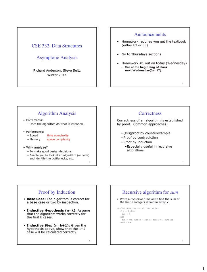
Announcements • Homework requires you get the textbook (either E2 or E3) CSE 332: Data Structures • Go to Thursdays sections Asymptotic Analysis • Homework #1 out on today (Wednesday) – Due at the beginning of class Richard Anderson, Steve Seitz next Wednesday (Jan 17). Winter 2014 2 Algorithm Analysis Correctness Correctness of an algorithm is established • Correctness: – Does the algorithm do what is intended. by proof. Common approaches: • Performance: – (Dis)proof by counterexample – Speed time complexity – Proof by contradiction – Memory space complexity – Proof by induction • Especially useful in recursive • Why analyze? algorithms – To make good design decisions – Enable you to look at an algorithm (or code) and identify the bottlenecks, etc. 3 4 Proof by Induction Recursive algorithm for sum • Base Case: The algorithm is correct for • Write a recursive function to find the sum of a base case or two by inspection. the first n integers stored in array v . sum(int array v, int n) returns int • Inductive Hypothesis (n=k): Assume if n = 0 then that the algorithm works correctly for sum = 0 the first k cases. else sum = nth number + sum of first n-1 numbers return sum • Inductive Step (n=k+1): Given the hypothesis above, show that the k+1 case will be calculated correctly. 5 6 1

Program Correctness by Induction How to measure performance? • Base Case: • Inductive Hypothesis (n=k): • Inductive Step (n=k+1): 7 8 Complexity cases Analyzing Performance We’ll start by focusing on two cases. We will focus on analyzing time complexity. First, we have some “rules” to help measure how long it takes to do things: Problem size N Basic operations Constant time – Worst-case complexity : max # steps Consecutive statements Sum of times algorithm takes on “most challenging” input Conditionals Test, plus larger branch cost of size N Loops Sum of iterations – Best-case complexity: min # steps Function calls Cost of function body algorithm takes on “easiest” input of size N Recursive functions Solve recurrence relation… Second, we will be interested in best and worst case performance. 9 9 10 Exercise - Searching Linear Search Analysis 2 3 5 16 37 50 73 75 bool LinearArrayContains (int array[], int n, int key ) { for( int i = 0; i < n; i++ ) { if( array[i] == key ) bool ArrayContains (int array[], int n, int key){ // Found it! Best Case: // Insert your algorithm here return true; } return false; Worst Case: } } What algorithm would you choose 11 12 to implement this code snippet? 2

Binary Search Analysis Solving Recurrence Relations 2 3 5 16 37 50 73 75 1. Determine the recurrence relation and base case(s). bool BinArrayContains ( int array[], int low, int high, int key ) { // The subarray is empty if( low > high ) return false; Best case: 2. “Expand” the original relation to find an equivalent // Search this subarray recursively expression in terms of the number of expansions (k) . int mid = (high + low) / 2; if( key == array[mid] ) { return true; } else if( key < array[mid] ) { return BinArrayFind ( array, low, mid-1, key ); Worst case: } else { return BinArrayFind ( array, mid+1, high, key ); } 3. Find a closed-form expression by setting k to a value which reduces the problem to a base case 13 14 Linear search — empirical analysis Linear Search vs Binary Search Linear Search Binary Search Best Case 4 5 at [middle] Worst Case 3n+3 7  log n  + 9 time (# ops) N (= array size) Each search produces a dot in above graph. 15 16 Blue = less frequently occurring, Red = more frequent Binary search — empirical analysis Empirical comparison time (# ops) time (# ops) N (= array size) N (= array size) Linear search Binary search Gives additional information N (= array size) Each search produces a dot in above graph. 17 18 Blue = less frequently occurring, Red = more frequent 3

Fast Computer vs. Smart Programmer Fast Computer vs. Slow Computer (small data) 19 20 Fast Computer vs. Smart Programmer Asymptotic Analysis (big data) • Consider only the order of the running time – A valuable tool when the input gets “large” – Ignores the effects of different machines or different implementations of same algorithm 21 22 Asymptotic Analysis Asymptotic Analysis • To find the asymptotic runtime, throw Eliminate low order terms away the constants and low-order – 4n + 5  terms – 0.5 n log n + 2n + 7  – n 3 + 3 2 n + 8n  – Linear search is    T LS ( n ) 3 n 3 O ( n ) worst      Eliminate coefficients – Binary search is T BS ( n ) 7 log n 9 O (log n ) worst 2 – 4n  – 0.5 n log n  Remember: the “fastest” algorithm has the – 3 2 n => slowest growing function for its runtime 23 24 4

Properties of Logs Properties of Logs Basic: Changing base  multiply by constant • A logAB = B – For example: log 2 x = 3.22 log 10 x • log A A = – More generally Independent of base: • log(AB) =   1    log n log n   A B  log A  B • log(A/B) = – Means we can ignore the base for • log(A B ) = asymptotic analysis (since we’re ignoring constant multipliers) • log((A B ) C ) = 25 26 Another example Comparing functions • Eliminate • f(n) is an upper bound for h(n) 16 n 3 log 8 (10n 2 ) + 100n 2 low-order if h(n) ≤ f(n) for all n terms • Eliminate This is too strict – we mostly care about large n constant coefficients Still too strict if we want to ignore scale factors 27 28 Order Notation: Intuition Definition of Order Notation • h(n) є O(f(n)) Big- O “Order” if there exist positive constants c and n 0 such that h(n) ≤ c f(n) for all n ≥ n 0 a ( n ) = n 3 + 2 n 2 b ( n ) = 100 n 2 + 1000 O(f(n)) defines a class (set) of functions Although not yet apparent, as n gets “sufficiently large”, a ( n ) will be “greater than or equal to” b ( n ) 29 30 5

Order Notation: Example Example h ( n )  O( f ( n ) ) iff there exist positive constants c and n 0 such that: h ( n )  c f ( n ) for all n  n 0 Example: 100 n 2 + 1000  1 ( n 3 + 2 n 2 ) for all n  100 So 100 n 2 + 1000  O( n 3 + 2 n 2 ) 100 n 2 + 1000  ( n 3 + 2 n 2 ) for all n  100 So 100 n 2 + 1000  O( n 3 + 2 n 2 ) 31 32 Constants are not unique Another Example: Binary Search h ( n )  O( f ( n ) ) iff there exist positive h ( n )  O( f ( n ) ) iff there exist positive constants c and n 0 such that: constants c and n 0 such that: h ( n )  c f ( n ) for all n  n 0 h ( n )  c f ( n ) for all n  n 0 Example: Is 7log 2 n + 9  O (log 2 n)? 100 n 2 + 1000  1 ( n 3 + 2 n 2 ) for all n  100 100 n 2 + 1000  1/2 ( n 3 + 2 n 2 ) for all n  198 33 34 Order Notation: Some Notes on Notation Worst Case Binary Search Sometimes you’ll see (e.g., in Weiss) h ( n ) = O( f ( n ) ) or h ( n ) is O( f ( n ) ) These are equivalent to h ( n )  O( f ( n ) ) 35 36 6

Big-O: Common Names Asymptotic Lower Bounds •  ( g ( n ) ) is the set of all functions asymptotically greater than or equal to g ( n ) – constant: O(1) – logarithmic: O(log n) (log k n, log n 2  O(log n)) – linear: O(n) • h ( n )   ( g( n ) ) iff – log-linear: O(n log n) There exist c >0 and n 0 >0 such that h ( n )  c – quadratic: O(n 2 ) g( n ) for all n  n 0 – cubic: O(n 3 ) – polynomial: O(n k ) (k is a constant) – exponential: O(c n ) (c is a constant > 1) 37 38 Asymptotic Tight Bound Full Set of Asymptotic Bounds •  ( f ( n ) ) is the set of all functions • O( f ( n ) ) is the set of all functions asymptotically equal to f ( n ) asymptotically less than or equal to f ( n ) – o( f ( n ) ) is the set of all functions • h ( n )   ( f ( n ) ) iff asymptotically strictly less than f ( n ) h ( n )  O( f ( n ) ) and h ( n )   ( f ( n ) ) - This is equivalent to: •  ( g ( n ) ) is the set of all functions   lim ( )/ ( ) h n f n c 0  n asymptotically greater than or equal to g ( n ) –  ( g ( n ) ) is the set of all functions asymptotically strictly greater than g ( n ) •  ( f ( n ) ) is the set of all functions asymptotically equal to f ( n ) 39 40 Big-Omega et al. Intuitively Formal Definitions • h ( n )  O( f ( n ) ) iff There exist c >0 and n 0 >0 such that h ( n )  c f ( n ) for all n  n 0 Asymptotic Notation Mathematics • h ( n )  o( f ( n ) ) iff There exists an n 0 >0 such that h ( n ) < c f ( n ) for all c >0 and n  n 0 Relation – This is equivalent to:  lim ( )/ ( ) h n f n 0 O   n • h ( n )   ( g( n ) ) iff   There exist c >0 and n 0 >0 such that h ( n )  c g( n ) for all n  n 0  = • h ( n )   ( g( n ) ) iff There exists an n 0 >0 such that h ( n ) > c g( n ) for all c >0 and n  n 0 o < – This is equivalent to:   lim ( )/ ( ) h n g n  >  n • h ( n )   ( f ( n ) ) iff h ( n )  O( f ( n ) ) and h ( n )   ( f ( n ) ) – This is equivalent to:   lim ( )/ ( ) h n f n c 0  n 41 42 7