CSE 332: Data Structures Homework 1, Wednesday, beginning of - PDF document

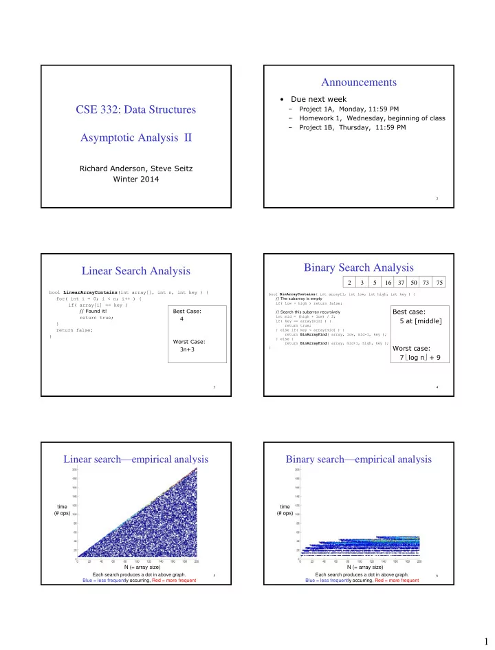
Announcements • Due next week – Project 1A, Monday, 11:59 PM CSE 332: Data Structures – Homework 1, Wednesday, beginning of class – Project 1B, Thursday, 11:59 PM Asymptotic Analysis II Richard Anderson, Steve Seitz Winter 2014 2 Binary Search Analysis Linear Search Analysis 2 3 5 16 37 50 73 75 bool LinearArrayContains (int array[], int n, int key ) { bool BinArrayContains ( int array[], int low, int high, int key ) { for( int i = 0; i < n; i++ ) { // The subarray is empty if( low > high ) return false; if( array[i] == key ) Best Case: Best case: // Found it! // Search this subarray recursively int mid = (high + low) / 2; return true; 4 5 at [middle] if( key == array[mid] ) { } return true; return false; } else if( key < array[mid] ) { return BinArrayFind ( array, low, mid-1, key ); } } else { Worst Case: return BinArrayFind ( array, mid+1, high, key ); Worst case: 3n+3 } 7  log n  + 9 3 4 Linear search — empirical analysis Binary search — empirical analysis time time (# ops) (# ops) N (= array size) N (= array size) Each search produces a dot in above graph. Each search produces a dot in above graph. 5 6 Blue = less frequently occurring, Red = more frequent Blue = less frequently occurring, Red = more frequent 1

Fast Computer vs. Slow Computer Empirical comparison time (# ops) N (= array size) N (= array size) Linear search Binary search Gives additional information 7 8 Fast Computer vs. Smart Programmer Fast Computer vs. Smart Programmer (big data) (small data) 9 10 Asymptotic Analysis Asymptotic Analysis • To find the asymptotic runtime, throw • Consider only the order of the running time away the constants and low-order terms – A valuable tool when the input gets “large” – Ignores the effects of different machines or – Linear search is    T LS ( n ) 3 n 3 O ( n ) different implementations of same algorithm worst      – Binary search is T BS ( n ) 7 log n 9 O (log n ) worst 2 Remember: the “fastest” algorithm has the slowest growing function for its runtime 11 12 2

Asymptotic Analysis Properties of Logs Basic: Eliminate low order terms • A logAB = B – 4n + 5  • log A A = – 0.5 n log n + 2n + 7  – n 3 + 3 2 n + 8n  Independent of base: • log(AB) = Eliminate coefficients • log(A/B) = – 4n  – 0.5 n log n  • log(A B ) = – 3 2 n => • log((A B ) C ) = 13 14 Properties of Logs Another example • Eliminate Changing base  multiply by constant 16 n 3 log 8 (10n 2 ) + 100n 2 low-order – For example: log 2 x = 3.22 log 10 x terms – More generally • Eliminate constant   1    log n   log n coefficients A B  log A  B – Means we can ignore the base for asymptotic analysis (since we’re ignoring constant multipliers) 15 16 Comparing functions Definition of Order Notation • f(n) is an upper bound for h(n) • h(n) є O(f(n)) Big- O “Order” if h(n) ≤ f(n) for all n if there exist positive constants c and n 0 such that h(n) ≤ c f(n) for all n ≥ n 0 This is too strict – we mostly care about large n O(f(n)) defines a class (set) of functions Still too strict if we want to ignore scale factors 17 18 3

Order Notation: Intuition Order Notation: Example a ( n ) = n 3 + 2 n 2 b ( n ) = 100 n 2 + 1000 Although not yet apparent, as n gets “sufficiently 100 n 2 + 1000  ( n 3 + 2 n 2 ) for all n  100 large”, a ( n ) will be “greater than or equal to” b ( n ) So 100 n 2 + 1000  O( n 3 + 2 n 2 ) 19 20 Example Constants are not unique h ( n )  O( f ( n ) ) iff there exist positive h ( n )  O( f ( n ) ) iff there exist positive constants c and n 0 such that: constants c and n 0 such that: h ( n )  c f ( n ) for all n  n 0 h ( n )  c f ( n ) for all n  n 0 Example: Example: 100 n 2 + 1000  1 ( n 3 + 2 n 2 ) for all n  100 100 n 2 + 1000  1 ( n 3 + 2 n 2 ) for all n  100 So 100 n 2 + 1000  O( n 3 + 2 n 2 ) 100 n 2 + 1000  1/2 ( n 3 + 2 n 2 ) for all n  198 21 22 Order Notation: Another Example: Binary Search Worst Case Binary Search h ( n )  O( f ( n ) ) iff there exist positive constants c and n 0 such that: h ( n )  c f ( n ) for all n  n 0 Is 7log 2 n + 9  O (log 2 n)? 23 24 4

Some Notes on Notation Big-O: Common Names Sometimes you’ll see (e.g., in Weiss) – constant: O(1) – logarithmic: O(log n) (log k n, log n 2  O(log n)) h ( n ) = O( f ( n ) ) – linear: O(n) – log-linear: O(n log n) or – quadratic: O(n 2 ) – cubic: O(n 3 ) h ( n ) is O( f ( n ) ) – polynomial: O(n k ) (k is a constant) – exponential: O(c n ) (c is a constant > 1) These are equivalent to h ( n )  O( f ( n ) ) 25 26 Asymptotic Lower Bounds Asymptotic Tight Bound •  ( g ( n ) ) is the set of all functions •  ( f ( n ) ) is the set of all functions asymptotically greater than or equal to g ( n ) asymptotically equal to f ( n ) • h ( n )   ( f ( n ) ) iff • h ( n )   ( g( n ) ) iff h ( n )  O( f ( n ) ) and h ( n )   ( f ( n ) ) There exist c >0 and n 0 >0 such that h ( n )  c - This is equivalent to: g( n ) for all n  n 0   lim ( )/ ( ) h n f n c 0  n 27 28 Full Set of Asymptotic Bounds Formal Definitions • h ( n )  O( f ( n ) ) iff • O( f ( n ) ) is the set of all functions There exist c >0 and n 0 >0 such that h ( n )  c f ( n ) for all n  n 0 asymptotically less than or equal to f ( n ) • h ( n )  o( f ( n ) ) iff – o( f ( n ) ) is the set of all functions There exists an n 0 >0 such that h ( n ) < c f ( n ) for all c >0 and n  n 0 asymptotically strictly less than f ( n ) – This is equivalent to:  lim ( )/ ( ) h n f n 0  n • h ( n )   ( g( n ) ) iff •  ( g ( n ) ) is the set of all functions There exist c >0 and n 0 >0 such that h ( n )  c g( n ) for all n  n 0 asymptotically greater than or equal to g ( n ) • h ( n )   ( g( n ) ) iff –  ( g ( n ) ) is the set of all functions There exists an n 0 >0 such that h ( n ) > c g( n ) for all c >0 and n  n 0 asymptotically strictly greater than g ( n ) – This is equivalent to:   lim ( )/ ( ) h n g n  n • h ( n )   ( f ( n ) ) iff h ( n )  O( f ( n ) ) and h ( n )   ( f ( n ) ) •  ( f ( n ) ) is the set of all functions – This is equivalent to:   lim ( )/ ( ) h n f n c 0 asymptotically equal to f ( n )  n 29 30 5

Big-Omega et al. Intuitively Complexity cases (revisited) Problem size N – Worst-case complexity : max # steps Asymptotic Notation Mathematics algorithm takes on “most challenging” input Relation of size N – Best-case complexity: min # steps O  algorithm takes on “easiest” input of size N    = – Average-case complexity : avg # steps o < algorithm takes on random inputs of size N – Amortized complexity : max total # steps  > algorithm takes on M “most challenging” consecutive inputs of size N , divided by M (i.e., divide the max total by M ). 31 32 Bounds vs. Cases Bounds vs. Cases Two orthogonal axes: – Bound Flavor • Upper bound (O, o) • Lower bound (  ,  ) • Asymptotically tight (  ) – Analysis Case • Worst Case (Adversary), T worst ( n ) • Average Case, T avg ( n ) • Best Case, T best ( n ) • Amortized, T amort ( n ) One can estimate the bounds for any given case. 33 34 Pros and Cons Big-Oh Caveats of Asymptotic Analysis • Asymptotic complexity (Big-Oh) considers only large n – You can “abuse” it to be misled about trade -offs – Example: n 1/10 vs. log n • Asymptotically n 1/10 grows more quickly • But the “cross - over” point is around 5 * 10 17 • So n 1/10 better for almost any real problem • Comparing O() for small n values can be misleading – Quicksort: O(nlogn) – Insertion Sort: O(n 2 ) – Yet in reality Insertion Sort is faster for small n – We’ll learn about these sorts later 35 36 6