2012 07 10
play

2012-07-10 CSE 332 Data Abstractions: B Trees and Hash Tables Make - PDF document

2012-07-10 CSE 332 Data Abstractions: B Trees and Hash Tables Make a Complete Breakfast The national data structure of the Netherlands HASH TABLES Kate Deibel Summer 2012 July 9, 2012 CSE 332 Data Abstractions, Summer 2012 1 July 9, 2012


  1. 2012-07-10 CSE 332 Data Abstractions: B Trees and Hash Tables Make a Complete Breakfast The national data structure of the Netherlands HASH TABLES Kate Deibel Summer 2012 July 9, 2012 CSE 332 Data Abstractions, Summer 2012 1 July 9, 2012 CSE 332 Data Abstractions, Summer 2012 2 Hash Tables An Ideal Hash Functions A hash table is an array of some fixed size  Is fast to compute Basic idea:  Rarely hashes two keys to the same index hash table 0  Known as collisions  Zero collisions often impossible in theory but reasonably achievable in practice hash function: 0 index = h(key) ⁞ key space (e.g., integers, strings) ⁞ hash function: index = h(key) size -1 The goal: Aim for constant-time find, insert, and delete "on key space (e.g., integers, strings) average" under reasonable assumptions size -1 July 9, 2012 CSE 332 Data Abstractions, Summer 2012 3 July 9, 2012 CSE 332 Data Abstractions, Summer 2012 4 What to Hash? Hashing Integers key space = integers We will focus on two most common things to hash: ints and strings Simple hash function: 0 If you have objects with several fields, it is h(key) = key % TableSize 10 1 usually best to hash most of the "identifying 41 2 fields" to avoid collisions:  Client: f(x) = x 3  Library: g(x) = f(x) % TableSize class Person { 4  Fairly fast and natural String firstName, middleName, lastName; 34 5 Date birthDate; 6 … Example: use these four values
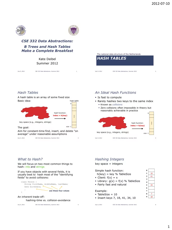
 7 }  TableSize = 10 7 8 An inherent trade-off: 18 9  Insert keys 7, 18, 41, 34, 10 hashing-time vs. collision-avoidance July 9, 2012 CSE 332 Data Abstractions, Summer 2012 5 July 9, 2012 CSE 332 Data Abstractions, Summer 2012 6 1

  2. 2012-07-10 Hashing non-integer keys Hashing Strings If keys are not ints, the client must provide a Key space K = s 0 s 1 s 2 …s k-1 where s i are chars: s i  [0, 256] means to convert the key to an int Some choices: Which ones best avoid collisions? Programming Trade-off:  Calculation speed h K = s 0 % TableSize  Avoiding distinct keys hashing to same ints k−1 h K = s i % TableSize i=0 k−1 s i ∙ 37 𝑗 % TableSize h K = i=0 July 9, 2012 CSE 332 Data Abstractions, Summer 2012 7 July 9, 2012 CSE 332 Data Abstractions, Summer 2012 8 Combining Hash Functions A few rules of thumb / tricks: 1. Use all 32 bits (be careful with negative numbers) 2. Use different overlapping bits for different parts of the hash  This is why a factor of 37 i works better than 256 i  Example: "abcde" and "ebcda" 3. When smashing two hashes into one hash, use bitwise-xor  bitwise-and produces too many 0 bits  bitwise-or produces too many 1 bits Calling a State Farm agent is not an option… COLLISION RESOLUTION 4. Rely on expertise of others; consult books and other resources for standard hashing functions 5. Advanced: If keys are known ahead of time, a perfect hash can be calculated July 9, 2012 CSE 332 Data Abstractions, Summer 2012 9 July 9, 2012 CSE 332 Data Abstractions, Summer 2012 10 Collision Avoidance Collision Resolution With (x%TableSize), number of collisions depends on Collision:  the ints inserted When two keys map to the same location  TableSize in the hash table Larger table-size tends to help, but not always  Example: 70, 24, 56, 43, 10 We try to avoid it, but the number of keys with TableSize = 10 and TableSize = 60 always exceeds the table size Technique: Pick table size to be prime. Why?  Real-life data tends to have a pattern, Ergo, hash tables generally must support  "Multiples of 61" are probably less likely than some form of collision resolution "multiples of 60"  Some collision strategies do better with prime size July 9, 2012 CSE 332 Data Abstractions, Summer 2012 11 July 9, 2012 CSE 332 Data Abstractions, Summer 2012 12 2

  3. 2012-07-10 Flavors of Collision Resolution Terminology Warning Separate Chaining We and the book use the terms  "chaining" or "separate chaining"  "open addressing " Open Addressing  Linear Probing Very confusingly, others use the terms  "open hashing" for "chaining"  Quadratic Probing  "closed hashing" for "open addressing"  Double Hashing We also do trees upside-down July 9, 2012 CSE 332 Data Abstractions, Summer 2012 13 July 9, 2012 CSE 332 Data Abstractions, Summer 2012 14 Separate Chaining Separate Chaining All keys that map to the same All keys that map to the same table location are kept in a linked table location are kept in a linked 0 / 0 10 / list (a.k.a. a "chain" or "bucket") list (a.k.a. a "chain" or "bucket") 1 / 1 / 2 / 2 / 3 / 3 / 4 / As easy as it sounds 4 / As easy as it sounds 5 / 5 / 6 / 6 / 7 / 7 / Example: Example: 8 / 8 / insert 10, 22, 86, 12, 42 insert 10, 22, 86, 12, 42 9 / 9 / with h(x) = x % 10 with h(x) = x % 10 July 9, 2012 CSE 332 Data Abstractions, Summer 2012 15 July 9, 2012 CSE 332 Data Abstractions, Summer 2012 16 Separate Chaining Separate Chaining All keys that map to the same All keys that map to the same table location are kept in a linked table location are kept in a linked 0 10 / 0 10 / list (a.k.a. a "chain" or "bucket") list (a.k.a. a "chain" or "bucket") 1 / 1 / 2 2 22 / 22 / 3 / 3 / 4 / As easy as it sounds 4 / As easy as it sounds 5 / 5 / 86 / 6 / 6 7 / 7 / Example: Example: 8 / 8 / insert 10, 22, 86, 12, 42 insert 10, 22, 86, 12, 42 9 / 9 / with h(x) = x % 10 with h(x) = x % 10 July 9, 2012 CSE 332 Data Abstractions, Summer 2012 17 July 9, 2012 CSE 332 Data Abstractions, Summer 2012 18 3

  4. 2012-07-10 Separate Chaining Separate Chaining All keys that map to the same All keys that map to the same table location are kept in a linked table location are kept in a linked 0 10 / 0 10 / list (a.k.a. a "chain" or "bucket") list (a.k.a. a "chain" or "bucket") 1 / 1 / 2 12 22 / 2 42 12 22 / 3 / 3 / 4 / As easy as it sounds 4 / As easy as it sounds 5 / 5 / 6 86 / 6 86 / 7 / 7 / Example: Example: 8 / 8 / insert 10, 22, 86, 12, 42 insert 10, 22, 86, 12, 42 9 / 9 / with h(x) = x % 10 with h(x) = x % 10 July 9, 2012 CSE 332 Data Abstractions, Summer 2012 19 July 9, 2012 CSE 332 Data Abstractions, Summer 2012 20 Thoughts on Separate Chaining Rigorous Separate Chaining Analysis Worst-case time for find? The load factor,  , of a hash table is calculated as 𝑜  Linear 𝜇 = 𝑈𝑏𝑐𝑚𝑓𝑇𝑗𝑨𝑓 But only with really bad luck or bad hash function  where n is the number of items currently in the table  Not worth avoiding (e.g., with balanced trees at each bucket)  Keep small number of items in each bucket  Overhead of tree balancing not worthwhile for small n Beyond asymptotic complexity, some "data-structure engineering" can improve constant factors  Linked list, array, or a hybrid Insert at end or beginning of list   Sorting the lists gains and loses performance Splay-like: Always move item to front of list  July 9, 2012 CSE 332 Data Abstractions, Summer 2012 21 July 9, 2012 CSE 332 Data Abstractions, Summer 2012 22 Load Factor? Load Factor? 0 10 / 0 10 / 1 / 1 71 2 31 / 2 2 42 12 22 / 42 12 22 / 3 / 3 63 73 / 4 / 4 / 75 5 65 95 / 5 / 5 86 / 86 / 6 6 7 / 7 27 47 8 / 8 88 18 38 98 / 9 / 𝑜 = 5 9 99 / 𝑜 = 21 10 = 2.1 𝜇 = 𝑈𝑏𝑐𝑚𝑓𝑇𝑗𝑨𝑓 = ? 10 = 0.5 𝜇 = 𝑈𝑏𝑐𝑚𝑓𝑇𝑗𝑨𝑓 = ? July 9, 2012 CSE 332 Data Abstractions, Summer 2012 23 July 9, 2012 CSE 332 Data Abstractions, Summer 2012 24 4

Download Presentation
Download Policy: The content available on the website is offered to you 'AS IS' for your personal information and use only. It cannot be commercialized, licensed, or distributed on other websites without prior consent from the author. To download a presentation, simply click this link. If you encounter any difficulties during the download process, it's possible that the publisher has removed the file from their server.

Recommend


More recommend