CSE 326: Data Structures (amortized) linked list Array Hash - - PowerPoint PPT Presentation

1

1

CSE 326: Data Structures Hash Tables

Hal Perkins Spring 2007 Lecture 16

2

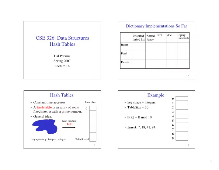
Dictionary Implementations So Far

Delete Find Insert Splay

(amortized)

AVL BST Sorted Array Unsorted linked list

3

Hash Tables

• Constant time accesses!
• A hash table is an array of some

fixed size, usually a prime number.

• General idea:

key space (e.g., integers, strings)

…

TableSize –1 hash function: h(K) hash table

4

Example

• key space = integers
• TableSize = 10
• h(K) = K mod 10
• Insert: 7, 18, 41, 94

2 3 9 8 7 6 5 4 1

2

5

Another Example

• key space = integers
• TableSize = 6
• h(K) = K mod 6
• Insert: 7, 18, 41, 34

2 3 5 4 1

6

Hash Functions

• 1. simple/fast to compute,
• 2. Avoid collisions
• 3. have keys distributed evenly among cells.

Perfect Hash function:

7

Sample Hash Functions:

• key space = strings
• s = s0 s1 s2 … s k-1

1. h(s) = s0 mod TableSize 2. h(s) = mod TableSize 3. h(s) = mod TableSize ⎟ ⎠ ⎞ ⎜ ⎝ ⎛ ∑

− = 1 k i i

s ⎟ ⎠ ⎞ ⎜ ⎝ ⎛ ⋅

∑

− = 1

37

k i i i

s

8

Collision Resolution

Collision: when two keys map to the same location in the hash table. Two ways to resolve collisions:

• 1. Separate Chaining
• 2. Open Addressing (linear probing,

quadratic probing, double hashing)

3

9

Separate Chaining

• Separate chaining:

All keys that map to the same hash value are kept in a list (or “bucket”).

2 3 9 8 7 6 5 4 1

Insert: 10 22 107 12 42

10

Analysis of find

• Defn: The load factor, λ, of a hash table is

the ratio: ← no. of elements ← table size For separate chaining, λ = average # of elements in a bucket

• Unsuccessful find:
• Successful find:

M N

11

How big should the hash table be?

• For Separate Chaining:

12

tableSize: Why Prime?

• Suppose

– data stored in hash table: 7160, 493, 60, 55, 321, 900, 810 – tableSize = 10 data hashes to 0, 3, 0, 5, 1, 0, 0 – tableSize = 11 data hashes to 10, 9, 5, 0, 2, 9, 7

Real-life data tends to have a pattern Being a multiple of 11 is usually not the pattern ☺

4

13

Open Addressing

2 3 9 8 7 6 5 4 1

Insert: 38 19 8 109 10

• Linear Probing:

after checking spot h(k), try spot h(k)+1, if that is full, try h(k)+2, then h(k)+3, etc.

14

Terminology Alert!

“Open Hashing” equals “Separate Chaining” “Closed Hashing” equals “Open Addressing”

Weiss

15

Linear Probing

f(i) = i

• Probe sequence:

0th probe = h(k) mod TableSize 1th probe = (h(k) + 1) mod TableSize 2th probe = (h(k) + 2) mod TableSize . . . ith probe = (h(k) + i) mod TableSize

16

Linear Probing – Clustering

[R. Sedgewick]

no collision no collision collision in small cluster collision in large cluster

5

17

Load Factor in Linear Probing

• For any λ < 1, linear probing will find an empty slot
• Expected # of probes (for large table sizes)

– successful search: – unsuccessful search:

• Linear probing suffers from primary clustering
• Performance quickly degrades for λ > 1/2

( ) ⎟

⎟ ⎠ ⎞ ⎜ ⎜ ⎝ ⎛ − +

2

1 1 1 2 1 λ

( )⎟

⎟ ⎠ ⎞ ⎜ ⎜ ⎝ ⎛ − + λ 1 1 1 2 1

18

Quadratic Probing

f(i) = i2

• Probe sequence:

0th probe = h(k) mod TableSize 1th probe = (h(k) + 1) mod TableSize 2th probe = (h(k) + 4) mod TableSize 3th probe = (h(k) + 9) mod TableSize . . . ith probe = (h(k) + i2) mod TableSize

Less likely to encounter Primary Clustering

19

Quadratic Probing

2 3 9 8 7 6 5 4 1

Insert: 89 18 49 58 79

20

Quadratic Probing Example

76

3 2 1 6 5 4

insert(76)

76%7 = 6

insert(40)

40%7 = 5

insert(48)

48%7 = 6

insert(5)

5%7 = 5

insert(55)

55%7 = 6

insert(47)

47%7 = 5

But…

6

21

Quadratic Probing: Success guarantee for λ < ½

• If size is prime and λ < ½, then quadratic probing will

find an empty slot in size/2 probes or fewer.

– show for all 0 ≤ i,j ≤ size/2 and i ≠ j

(h(x) + i2) mod size ≠ (h(x) + j2) mod size

– by contradiction: suppose that for some i ≠ j:

(h(x) + i2) mod size = (h(x) + j2) mod size ⇒ i2 mod size = j2 mod size ⇒ (i2 - j2) mod size = 0 ⇒ [(i + j)(i - j)] mod size = 0 BUT size does not divide (i-j) or (i+j)

22

Quadratic Probing: Properties

• For any λ < ½, quadratic probing will find an

empty slot; for bigger λ, quadratic probing may find a slot

• Quadratic probing does not suffer from primary

clustering: keys hashing to the same area are not bad

• But what about keys that hash to the same spot?

– Secondary Clustering!

23

Quadratic Probing Works for λ < 1/2

• If HSize is prime then

(h(x) + i2) mod HSize ≠ (h(x) + j2) mod HSize for i ≠ j and 0 < i,j < HSize/2.

• Proof

(h(x) + i2) mod HSize = (h(x) + j2) mod HSize (h(x) + i2) - (h(x) + j2) mod HSize = 0 (i2 - j2) mod HSize = 0 (i-j)(i+j) mod HSize = 0 ⇒⇐ HSize does not divide (i-j) or (i+j)

24

Double Hashing

f(i) = i * g(k) where g is a second hash function

• Probe sequence:

0th probe = h(k) mod TableSize 1th probe = (h(k) + g(k)) mod TableSize 2th probe = (h(k) + 2*g(k)) mod TableSize 3th probe = (h(k) + 3*g(k)) mod TableSize . . . ith probe = (h(k) + i*g(k)) mod TableSize

7

25

Double Hashing Example

1 2 3 4 5 6 76 76 1 2 3 4 5 6 93 76 93 1 2 3 4 5 6 93 40 76 40 1 2 3 4 5 6 47 93 40 76 47 1 2 3 4 5 6 47 93 10 40 76 10 1 2 3 4 5 6 47 93 10 55 40 76 55 h(k) = k mod 7 and g(k) = 5 – (k mod 5) Probes 1 1 1 2 1 2

26

Resolving Collisions with Double Hashing

2 3 9 8 7 6 5 4 1

Insert these values into the hash table in this order. Resolve any collisions with double hashing:

13 28 33 147 43

Hash Functions: H(K) = K mod M H2(K) = 1 + ((K/M) mod (M-1)) M =

27

Idea: When the table gets too full, create a bigger table (usually 2x as large) and hash all the items from the original table into the new table.

• When to rehash?

– half full (λ = 0.5) – when an insertion fails – some other threshold

• Cost of rehashing?

Rehashing

28

Java hashCode() Method

• Class Object defines a hashCode method

– Intent: returns a suitable hashcode for the object – Result is arbitrary int; must scale to fit a hash table (e.g. obj.hashCode() % nBuckets) – Used by collection classes like HashMap

• Classes should override with calculation

appropriate for instances of the class

– Calculation should involve semantically “significant” fields of objects

8

29

hashCode() and equals()

• To work right, particularly with collection

classes like HashMap, hashCode() and equals() must obey this rule: if a.equals(b) then it must be true that a.hashCode() == b.hashCode()

– Why?

• Reverse is not required

30

Hashing Summary

• Hashing is one of the most important data

structures.

• Hashing has many applications where
• perations are limited to find, insert, and

delete.

• Dynamic hash tables have good amortized

complexity.