CSCI 5832 Natural Language Processing Jim Martin Lecture 8 2/7/08 - - PDF document

1

2/7/08 1

CSCI 5832 Natural Language Processing

Jim Martin Lecture 8

2/7/08 2

Today 2/7

• Finish remaining LM issues

 Smoothing  Backoff and Interpolation

• Parts of Speech
• POS Tagging
• HMMs and Viterbi

2/7/08 3

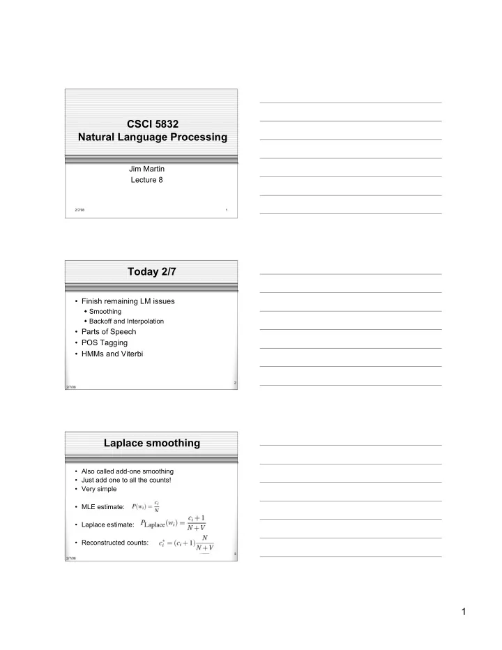
Laplace smoothing

• Also called add-one smoothing
• Just add one to all the counts!
• Very simple
• MLE estimate:
• Laplace estimate:
• Reconstructed counts:

2

2/7/08 4

Laplace smoothed bigram counts

2/7/08 5

Laplace-smoothed bigrams

2/7/08 6

Reconstituted counts

3

2/7/08 7

Big Changes to Counts

• C(count to) went from 608 to 238!
• P(to|want) from .66 to .26!
• Discount d= c*/c

 d for “chinese food” =.10!!! A 10x reduction  So in general, Laplace is a blunt instrument  Could use more fine-grained method (add-k)

• Despite its flaws Laplace (add-k) is however still used to

smooth other probabilistic models in NLP, especially

 For pilot studies  in domains where the number of zeros isn’t so huge.

2/7/08 8

Better Discounting Methods

• Intuition used by many smoothing

algorithms

 Good-Turing  Kneser-Ney  Witten-Bell

• Is to use the count of things we’ve seen
• nce to help estimate the count of things

we’ve never seen

2/7/08 9

Good-Turing

• Imagine you are fishing

 There are 8 species: carp, perch, whitefish, trout, salmon, eel, catfish, bass

• You have caught

 10 carp, 3 perch, 2 whitefish, 1 trout, 1 salmon, 1 eel = 18 fish (tokens) = 6 species (types)

• How likely is it that you’ll next see another trout?

4

2/7/08 10

Good-Turing

• Now how likely is it that next species is

new (i.e. catfish or bass)

3/18

There were 18 distinct events... 3 of those represent singleton species

2/7/08 11

Good-Turing

• But that 3/18s isn’t represented in our

probability mass. Certainly not the one we used for estimating another trout.

2/7/08 12

Good-Turing Intuition

• Notation: Nx is the frequency-of-frequency-x

 So N10=1, N1=3, etc

• To estimate total number of unseen species

 Use number of species (words) we’ve seen once  c0

* =c1 p0 = N1/N

• All other estimates are adjusted (down) to give

probabilities for unseen

Slide from Josh Goodman

5

2/7/08 13

Good-Turing Intuition

• Notation: Nx is the frequency-of-frequency-x

 So N10=1, N1=3, etc

• To estimate total number of unseen species

 Use number of species (words) we’ve seen once  c0* =c1 p0 = N1/N p0=N1/N=3/18

• All other estimates are adjusted (down) to give

probabilities for unseen

P(eel) = c*(1) = (1+1) 1/ 3 = 2/3 Slide from Josh Goodman

2/7/08 14

Bigram frequencies of frequencies and GT re-estimates

2/7/08 15

GT smoothed bigram probs

6

2/7/08 16

Backoff and Interpolation

• Another really useful source of knowledge
• If we are estimating:

 trigram p(z|xy)  but c(xyz) is zero

• Use info from:

 Bigram p(z|y)

• Or even:

 Unigram p(z)

• How to combine the trigram/bigram/unigram

info?

2/7/08 17

Backoff versus interpolation

• Backoff: use trigram if you have it,
• therwise bigram, otherwise unigram
• Interpolation: mix all three

2/7/08 18

Interpolation

• Simple interpolation
• Lambdas conditional on context:

7

2/7/08 19

How to set the lambdas?

• Use a held-out corpus
• Choose lambdas which maximize the

probability of some held-out data

 I.e. fix the N-gram probabilities  Then search for lambda values  That when plugged into previous equation  Give largest probability for held-out set  Can use EM to do this search

2/7/08 20

Practical Issues

• We do everything in log space

 Avoid underflow  (also adding is faster than multiplying)

2/7/08 21

Language Modeling Toolkits

• SRILM
• CMU-Cambridge LM Toolkit

8

2/7/08 22

Google N-Gram Release

2/7/08 23

Google N-Gram Release

• serve as the incoming 92
• serve as the incubator 99
• serve as the independent 794
• serve as the index 223
• serve as the indication 72
• serve as the indicator 120
• serve as the indicators 45
• serve as the indispensable 111
• serve as the indispensible 40
• serve as the individual 234

2/7/08 24

LM Summary

• Probability

 Basic probability  Conditional probability  Bayes Rule

• Language Modeling (N-grams)

 N-gram Intro  The Chain Rule

• Perplexity

 Smoothing:

• Add-1
• Good-Turing

9

2/7/08 25

Break

• Moving quiz to Thursday (2/14)
• Readings

 Chapter 2: All  Chapter 3:

• Skip 3.4.1 and 3.12

 Chapter 4

• Skip 4.7, 4.9, 4.10 and 4.11

 Chapter 5

• Read 5.1 through 5.5

2/7/08 26

Outline

• Probability
• Part of speech tagging

 Parts of speech  Tag sets  Rule-based tagging  Statistical tagging

• Simple most-frequent-tag baseline

 Important Ideas

• Training sets and test sets
• Unknown words
• Error analysis

 HMM tagging

2/7/08 27

Part of Speech tagging

• Part of speech tagging

 Parts of speech  What’s POS tagging good for anyhow?  Tag sets  Rule-based tagging  Statistical tagging

• Simple most-frequent-tag baseline

 Important Ideas

• Training sets and test sets
• Unknown words

 HMM tagging

10

2/7/08 28

Parts of Speech

• 8 (ish) traditional parts of speech

 Noun, verb, adjective, preposition, adverb, article, interjection, pronoun, conjunction, etc  Called: parts-of-speech, lexical category, word classes, morphological classes, lexical tags, POS  Lots of debate in linguistics about the number, nature, and universality of these

• We’ll completely ignore this debate.

2/7/08 29

POS examples

• N

noun chair, bandwidth, pacing

• V

verb study, debate, munch

• ADJ

adjective purple, tall, ridiculous

• ADV

adverb unfortunately, slowly

• P

preposition

• f, by, to
• PRO

pronoun I, me, mine

• DET

determiner the, a, that, those

2/7/08 30

POS Tagging: Definition

• The process of assigning a part-of-speech
• r lexical class marker to each word in a

corpus:

the koala put the keys

• n

the table

WORDS TAGS

N V P DET

11

2/7/08 31

POS Tagging example

WORD tag the DET koala N put V the DET keys N

• n

P the DET table N

2/7/08 32

What is POS tagging good for?

• First step of a vast number of practical tasks
• Speech synthesis

 How to pronounce “lead”?  INsult inSULT  OBject

• bJECT

 OVERflow

• verFLOW

 DIScount disCOUNT  CONtent conTENT

• Parsing

 Need to know if a word is an N or V before you can parse

• Information extraction

 Finding names, relations, etc.

• Machine Translation

2/7/08 33

Open and Closed Classes

• Closed class: a relatively fixed membership

 Prepositions: of, in, by, …  Auxiliaries: may, can, will had, been, …  Pronouns: I, you, she, mine, his, them, …  Usually function words (short common words which play a role in grammar)

• Open class: new ones can be created all the

time

 English has 4: Nouns, Verbs, Adjectives, Adverbs  Many languages have these 4, but not all!

12

2/7/08 34

Open class words

• Nouns

 Proper nouns (Boulder, Granby, Eli Manning)

• English capitalizes these.

 Common nouns (the rest).  Count nouns and mass nouns

• Count: have plurals, get counted: goat/goats, one goat, two goats
• Mass: don’t get counted (snow, salt, communism) (*two snows)
• Adverbs: tend to modify things

 Unfortunately, John walked home extremely slowly yesterday  Directional/locative adverbs (here,home, downhill)  Degree adverbs (extremely, very, somewhat)  Manner adverbs (slowly, slinkily, delicately)

• Verbs:

 In English, have morphological affixes (eat/eats/eaten)

2/7/08 35

Closed Class Words

• Idiosyncratic
• Examples:

 prepositions: on, under, over, …  particles: up, down, on, off, …  determiners: a, an, the, …  pronouns: she, who, I, ..  conjunctions: and, but, or, …  auxiliary verbs: can, may should, …  numerals: one, two, three, third, …

2/7/08 36

Prepositions from CELEX

13

2/7/08 37

English particles

2/7/08 38

Conjunctions

2/7/08 39

POS tagging: Choosing a tagset

• There are so many parts of speech, potential distinctions

we can draw

• To do POS tagging, need to choose a standard set of

tags to work with

• Could pick very coarse tagets

 N, V, Adj, Adv.

• More commonly used set is finer grained, the “UPenn

TreeBank tagset”, 45 tags

 PRP$, WRB, WP$, VBG

• Even more fine-grained tagsets exist

14

2/7/08 40

Penn TreeBank POS Tag set

2/7/08 41

Using the UPenn tagset

• The/DT grand/JJ jury/NN

commmented/VBD on/IN a/DT number/NN

• f/IN other/JJ topics/NNS ./.
• Prepositions and subordinating

conjunctions marked IN (“although/IN I/PRP..”)

• Except the preposition/complementizer

“to” is just marked “TO”.

2/7/08 42

POS Tagging

• Words often have more than one POS:

back

 The back door = JJ  On my back = NN  Win the voters back = RB  Promised to back the bill = VB

• The POS tagging problem is to determine

the POS tag for a particular instance of a word.

These examples from Dekang Lin

15

2/7/08 43

How hard is POS tagging? Measuring ambiguity

2/7/08 44

2 methods for POS tagging

• 1. Rule-based tagging

 (ENGTWOL)

• 2. Stochastic (=Probabilistic) tagging

 HMM (Hidden Markov Model) tagging

2/7/08 45

Rule-based tagging

• Start with a dictionary
• Assign all possible tags to words from the

dictionary

• Write rules by hand to selectively remove

tags

• Leaving the correct tag for each word.

16

2/7/08 46

Start with a dictionary

• she:

PRP

• promised:

VBN,VBD

• to

TO

• back:

VB, JJ, RB, NN

• the:

DT

• bill:

NN, VB

• Etc… for the ~100,000 words of English

2/7/08 47

Use the dictionary to assign every possible tag

NN RB VBN JJ VB PRP VBD TO VB DT NN She promised to back the bill

2/7/08 48

Write rules to eliminate tags

Eliminate VBN if VBD is an option when VBN|VBD follows “<start> PRP” NN RB JJ VB PRP VBD TO VB DT NN She promised to back the bill

VBN

17

2/7/08 49

Stage 1 of ENGTWOL Tagging

• First Stage: Run words through FST morphological

analyzer to get all parts of speech.

• Example: Pavlov had shown that salivation …

Pavlov PAVLOV N NOM SG PROPER had HAVE V PAST VFIN SVO HAVE PCP2 SVO shown SHOW PCP2 SVOO SVO SV that ADV PRON DEM SG DET CENTRAL DEM SG CS salivation N NOM SG

2/7/08 50

Stage 2 of ENGTWOL Tagging

• Second Stage: Apply NEGATIVE constraints.
• Example: Adverbial “that” rule

 Eliminates all readings of “that” except the one in

• “It isn’t that odd”

Given input: “that” If (+1 A/ADV/QUANT) ;if next word is adj/adv/quantifier (+2 SENT-LIM) ;following which is E-O-S (NOT -1 SVOC/A) ; and the previous word is not a ; verb like “consider” which ; allows adjective complements ; in “I consider that odd” Then eliminate non-ADV tags Else eliminate ADV

2/7/08 51

Hidden Markov Model Tagging

• Using an HMM to do POS tagging
• Is a special case of Bayesian inference

 Foundational work in computational linguistics  Bledsoe 1959: OCR  Mosteller and Wallace 1964: authorship identification

• It is also related to the “noisy channel”

model that’s the basis for ASR, OCR and MT

18

2/7/08 52

POS tagging as a sequence classification task

• We are given a sentence (an “observation” or

“sequence of observations”)

 Secretariat is expected to race tomorrow

• What is the best sequence of tags which

corresponds to this sequence of observations?

• Probabilistic view:

 Consider all possible sequences of tags  Out of this universe of sequences, choose the tag sequence which is most probable given the

• bservation sequence of n words w1…wn.

2/7/08 53

Getting to HMM

• We want, out of all sequences of n tags t1…tn the single

tag sequence such that P(t1…tn|w1…wn) is highest.

• Hat ^ means “our estimate of the best one”
• Argmaxx f(x) means “the x such that f(x) is maximized”

2/7/08 54

Getting to HMM

• This equation is guaranteed to give us the

best tag sequence

• But how to make it operational? How to

compute this value?

• Intuition of Bayesian classification:

 Use Bayes rule to transform into a set of other probabilities that are easier to compute

19

2/7/08 55

Using Bayes Rule

2/7/08 56

Likelihood and Prior

n

2/7/08 57

Two Kinds of probabilities (1)

• Tag transition probabilities p(ti|ti-1)

 Determiners likely to precede adjs and nouns

• That/DT flight/NN
• The/DT yellow/JJ hat/NN
• So we expect P(NN|DT) and P(JJ|DT) to be high
• But P(DT|JJ) to be:

 Compute P(NN|DT) by counting in a labeled corpus:

20

2/7/08 58

Two kinds of probabilities (2)

• Word likelihood probabilities p(wi|ti)

VBZ (3sg Pres verb) likely to be “is” Compute P(is|VBZ) by counting in a labeled corpus:

2/7/08 59

An Example: the verb “race”

• Secretariat/NNP is/VBZ expected/VBN to/TO

race/VB tomorrow/NR

• People/NNS continue/VB to/TO inquire/VB

the/DT reason/NN for/IN the/DT race/NN for/IN outer/JJ space/NN

• How do we pick the right tag?

2/7/08 60

Disambiguating “race”

21

2/7/08 61

Example

• P(NN|TO) = .00047
• P(VB|TO) = .83
• P(race|NN) = .00057
• P(race|VB) = .00012
• P(NR|VB) = .0027
• P(NR|NN) = .0012
• P(VB|TO)P(NR|VB)P(race|VB) = .00000027
• P(NN|TO)P(NR|NN)P(race|NN)=.00000000032
• So we (correctly) choose the verb reading,

2/7/08 62

Hidden Markov Models

• What we’ve described with these two

kinds of probabilities is a Hidden Markov Model

• Let’s just spend a bit of time tying this into

the model

• First some definitions.

2/7/08 63

Definitions

• A weighted finite-state automaton adds

probabilities to the arcs

 The sum of the probabilities leaving any arc must sum to one

• A Markov chain is a special case of a WFST in

which the input sequence uniquely determines which states the automaton will go through

• Markov chains can’t represent inherently

ambiguous problems

 Useful for assigning probabilities to unambiguous sequences

22

2/7/08 64

Markov chain for weather

2/7/08 65

Markov chain for words

2/7/08 66

Markov chain = “First-order

• bservable Markov Model”
• A set of states

 Q = q1, q2…qN; the state at time t is qt

• Transition probabilities:

 a set of probabilities A = a01a02…an1…ann.  Each aij represents the probability of transitioning from state i to state j  The set of these is the transition probability matrix A

• Current state only depends on previous state

23

2/7/08 67

Markov chain for weather

• What is the probability of 4 consecutive

rainy days?

• Sequence is rainy-rainy-rainy-rainy
• I.e., state sequence is 3-3-3-3
• P(3,3,3,3) =

 π1a11a11a11a11 = 0.2 x (0.6)3 = 0.0432

2/7/08 68

HMM for Ice Cream

• You are a climatologist in the year 2799
• Studying global warming
• You can’t find any records of the weather

in Baltimore, MA for summer of 2007

• But you find Jason Eisner’s diary
• Which lists how many ice-creams Jason

ate every date that summer

• Our job: figure out how hot it was

2/7/08 69

Hidden Markov Model

• For Markov chains, the output symbols are the

same as the states.

 See hot weather: we’re in state hot

• But in part-of-speech tagging (and other things)

 The output symbols are words  But the hidden states are part-of-speech tags

• So we need an extension!
• A Hidden Markov Model is an extension of a

Markov chain in which the input symbols are not the same as the states.

• This means we don’t know which state we are in.

24

2/7/08 70

• States Q = q1, q2…qN;
• Observations O= o1, o2…oN;

 Each observation is a symbol from a vocabulary V = {v1,v2,…vV}

• Transition probabilities

 Transition probability matrix A = {aij}

• Observation likelihoods

 Output probability matrix B={bi(k)}

• Special initial probability vector π

Hidden Markov Models

2/7/08 71

Eisner task

• Given

 Ice Cream Observation Sequence: 1,2,3,2,2,2,3…

• Produce:

 Weather Sequence: H,C,H,H,H,C…

2/7/08 72

HMM for ice cream

25

2/7/08 73

Transitions between the hidden states of HMM, showing A probs

2/7/08 74

B observation likelihoods for POS HMM