CSCE 970 Lecture 7: Earth, cant afford to visit each area to deter- - - PDF document

SLIDE 1

CSCE 970 Lecture 7: Clustering: Basic Concepts

Stephen D. Scott

March 23, 2001

1

Introduction

• What if labels unavailable?
• E.g. feat. vectors are measurements of elec-
• tromag. energy reflected from remote parts of

Earth, can’t afford to visit each area to deter- mine labels

• Clustering (a.k.a. unsupervised PR) algs. group

similar f.v.’s together based on a similarity measure

• If clustering is good, then can find label for
• ne of each group & use it as label for entire

group

Clustering Algorithm x1 x2 x1 x2 2

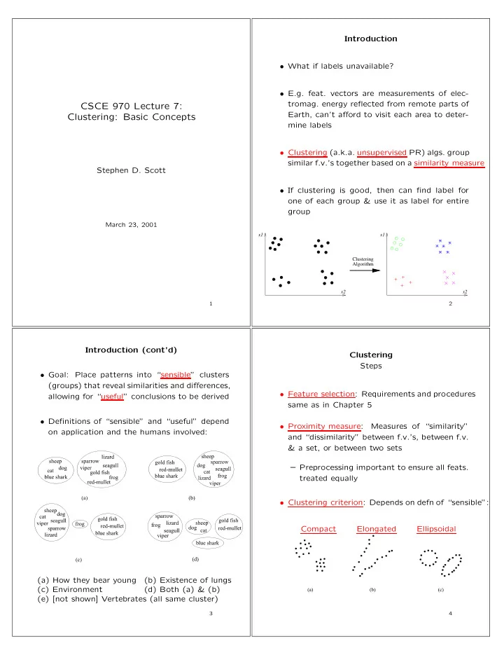
Introduction (cont’d)

• Goal: Place patterns into “sensible” clusters

(groups) that reveal similarities and differences, allowing for “useful” conclusions to be derived

• Definitions of “sensible” and “useful” depend
• n application and the humans involved:

(a) How they bear young (b) Existence of lungs (c) Environment (d) Both (a) & (b) (e) [not shown] Vertebrates (all same cluster)

3

Clustering Steps

• Feature selection: Requirements and procedures

same as in Chapter 5

• Proximity measure:

Measures of “similarity” and “dissimilarity” between f.v.’s, between f.v. & a set, or between two sets – Preprocessing important to ensure all feats. treated equally

• Clustering criterion: Depends on defn of “sensible”:

Compact Elongated Ellipsoidal

4

SLIDE 2

Clustering Steps (cont’d)

• Verify clustering tendency (Sec. 16.6)
• Clustering algorithm: Chapters 12–15
• Cluster validation: Verify that choices of alg.
• params. & cluster shape match data’s cluster-

ing structure (Chapt. 16)

• Interpretation:

The expert interprets results with other information

• Warning: Each step is subjective and depends
• n expert’s biases!

5

Clustering Applications

• Data reduction (compression): Represent each

cluster with single item

• Suggest hypotheses about nature of data
• Test hypotheses about data, e.g. that certain
• feats. are correlated while others are indepen-

dent

• Prediction based on groups: e.g. Slide 7.2

6

Clustering Types of Features

• Nominal: Name only, no quantitative compar-

isons possible, e.g. {male, female}

• Ordinal: Can be meaningfully ordered, but no

quantitative meaning on the differences, e.g. {4, 3, 2, 1} to represent {excellent, very good, good, poor}

• Interval-scaled: Difference is meaningful, ratio

is not, e.g. temperature measures on Celsius scale

• Ratio-scaled: Difference and ratio both mean-

ingful, e.g. weight

• Each type possesses the properties of the pre-

ceding types

7

Clustering Cluster Types

• Start with X = {x1, . . . , xN} and place into m

clusters C1, . . . , Cm

• Type 1: Hard (crisp)

Ci = ∅, i = 1, . . . , m

m

• i=1

Ci = X Ci ∩ Cj = ∅, i = j, i, j ∈ {1, . . . , m} – F.v.’s in Ci “more similar” to others in Ci than those in Cj, j = i

• Type 2: Fuzzy: Cj has membership function

µj : X → [0, 1] s.t.

m

• j=1

µj (xi) = 1, i ∈ {1, . . . , N} 0 <

N

• i=1

µj (xi) < N, j ∈ {1, . . . , m}

8

SLIDE 3

Proximity Measures Definitions

• Dissimilarity measure is func. d : X × X → ℜ s.t.

∃d0 ∈ ℜ : −∞ < d0 ≤ d(x, y) < +∞, ∀x, y ∈ X d(x, x) = d0 ∀x ∈ X d(x, y) = d(y, x) ∀x, y ∈ X

• d is a metric DM if d(x, y) = d0 ⇔ x = y

and d(x, z) ≤ d(x, y) + d(y, z) ∀x, y, z ∈ X – E.g. d2(·, ·) = Euclidean distance, d0 = 0

• Similarity measure is func. s : X × X → ℜ s.t.

∃s0 ∈ ℜ : −∞ < s(x, y) ≤ s0 < +∞, ∀x, y ∈ X s(x, x) = s0 ∀x ∈ X s(x, y) = s(y, x) ∀x, y ∈ X

• s is a metric SM if s(x, y) = s0 ⇔ x = y

and s(x, y) s(y, z) ≤ [s(x, y) + s(y, z)] s(x, z) ∀x, y, z ∈ X

9

Proximity Measures Definitions (cont’d)

• Can also define proximity measures between

sets of f.v.’s

• Let U = {D1, . . . , Dk}, Di ⊂ X,

PM α : U × U → ℜ

• E.g. X = {x1, x2, x3, x4, x5, x6}, U = {{x1, x2} ,

{x1, x4} , {x3, x4, x5} , {x1, x2, x3, x4, x5}}, dss

min

• Di, Dj
• =

min

x∈Di, y∈Dj

d2(x, y)

• Min. value is dss

min,0 = 0, dss min (Di, Di) = dss min,0,

and dss

min

• Di, Dj
• = dss

min

• Dj, Di
• , so dss

min(·, ·)

is a DM

• However, dss

min ({x1, x2} , {x1, x4}) = dss min,0 and

{x1, x2} = {x1, x4}, so not a metric DM

10

Proximity Measures Between Points Real-Valued Vectors Example Dissimilarity Measures (pp. 361–362)

• Common, general-purpose metric DM is weighted

Lp norm: dp(x, y) =

  ℓ

• i=1

wi |xi − yi|p

  1/p

• Special cases include weighted Euclidian dis-

tance (p = 2), weighted Manhattan distance d1(x, y) =

ℓ

• i=1

wi |xi − yi| , and weighted L∞ norm d∞(x, y) = max

1≤i≤ℓ {wi |xi − yi|}

• Generalization of weighted L2 norm is

d(x, y) =

• (x − y)TB (x − y) ,

e.g. Mahalanobis distance

11

Proximity Measures Between Points Real-Valued Vectors Example Similarity Measures (pp. 362–363)

• Inner product:

sinner(x, y) = xTy =

ℓ

• i=1

xi yi

• If x2, y2 ≤ a, then −a2 ≤ sinner(x, y) ≤ a2
• Tanimoto distance:

sT(x, y) = xT y x2

2 + y2 2 − xT y =

1 1 + (x−y)T (x−y)

xT y

, which is inversely prop. to (squared Euclid. dist.)/(correlation measure)

12

SLIDE 4

Proximity Measures Between Points Discrete-Valued Vectors

• If the coordinates of f.v.’s come from {0, . . . , k−

1}, can use SMs and DMs defined for real- valued f.v.’s, (e.g. weighted Lp norm) plus: – Hamming distance: DM measuring number

• f places where x and y differ

– Tanimoto measure: SM measuring number

• f places where x and y are same, divided

by total number of places ∗ Ignore places i where xi = yi = 0 · Useful for ordinal features where xi is degree to which x possesses ith feature

13

Proximity Measures Between Points Fuzzy Measures

• Let xi ∈ [0, 1] be measure of how much x pos-

sesses ith feature

• If xi, yi ∈ {0, 1}, then

(xi ≡ yi) = ((¬xi ∧ ¬yi) ∨ (xi ∧ yi))

• Generalize to fuzzy values:

s(xi, yi) = max {min {1 − xi, 1 − yi} , min {xi, yi}}

• To measure similarity between vectors:

sp

F(x, y) =   ℓ

• i=1

s(xi, yi)p

  1/p

• ℓ1/p

/2 ≤ sq

F (·, ·) ≤ ℓ1/p

• So s∞

F = max1≤i≤ℓ s(xi, yi) and

s1

F = ℓ i=1 s(xi, yi) = generalization of Ham-

ming distance

14

• Prox. Measures Between a Point and a Set
• Might want to measure proximity of point x to

existing cluster C

• Can measure proximity α by using all points of

C or by using a representative of C

• If all points of C used, common choices:

αps

max(x, C) = max y∈C {α(x, y)}

αps

min(x, C) = min y∈C {α(x, y)}

αps

avg(x, C) = 1

|C|

• y∈C

α(x, y) , where α(x, y) is any measure between x and y

15

• Prox. Measures Between a Point and a Set

Representatives

• Alternative: Measure distance between point

x and a representative of the set C

• Appropriate choice of representative depends
• n type of cluster

Compact Elongated Hyperspherical Point Hyperplane Hypersphere

16

SLIDE 5

• Prox. Measures Between a Point and a Set

Examples of Point Representatives

• Mean vector: mp = 1

|C|

• y∈C

y

• Works well in ℜℓ, but might not exist in dis-

crete space

• Mean center mc ∈ C:
• y∈C

d(mc, y) ≤

• y∈C

d(z, y) ∀z ∈ C , where d(·, ·) is DM (if SM used, reverse ineq.)

• Median center: For each point y ∈ C, find me-

dian dissimilarity from y to all other points of C, then take min; so mmed ∈ C is defined as medy∈C {d(mmed, y)} ≤ medy∈C {d(z, y)} ∀z ∈ C

• Examples p. 375
• Now can measure proximity between C’s rep

and x with standard measures

17

• Prox. Measures Between a Point and a Set

Hyperplane & Hyperspherical Representatives

• Definition of hyperplane H and dist. function:

aTx + a0 = 0 d(x, H) = min

z∈H d(x, z)

• Definition of hypersphere Q and dist. function:

(x − c)T(x − c) = r2 d(x, Q) = min

z∈Q d(x, z)

Hyperplane Hypersphere

• Given set of points, can find representative via

regression techniques, minimizing sum of dis- tances between points and representative

18

• Prox. Measures Between Two Sets
• Given sets of f.v.’s Di and Dj and prox. meas.

α(·, ·)

• Max: αss

max(Di, Dj) =

max

x∈Di,y∈Dj

{α(x, y)} is a measure (but not necessarily a metric) iff α is a SM – E.g. α is Euclid. dist. (a DM), ℓ = 1, D1 = {(1), (10)}, D2 = {(4), (7)}: αss

max(D1, D1) = 9 = 3 = αss max(D2, D2)

– α is SM ⇒ α(x, y) ≤ s0 ∀x, y and α(x, x) = s0 ∀x, so αss

max(Di, Dj) ≤ s0 ∀Di, Dj,

and ∀D αss

max(D, D) =

max

x∈D,y∈D {α(x, y)} = max x∈D {α(x, x)} = s0

αss

max(Di, Dj) = αss max(Dj, Di)

19

• Prox. Measures Between Two Sets

(cont’d)

• Min: αss

min(Di, Dj) =

min

x∈Di,y∈Dj

{α(x, y)} is a measure (but not a metric) iff α is a DM

• Average: αss

avg(Di, Dj) =

1 |Di| |Dj|

• x∈Di
• y∈Dj

α(x, y) is not necessarily a measure even if α is

• Representative (mean):

αss

rep(Di, Dj) = α(mDi, mDj),

(mDi is point rep. of Di) is a measure whenever α is

20

SLIDE 6

Overview of Clustering Algorithms Exhaustive Search

• Want to find set of clusters that maximizes

SM or minimizes DM

• Option 1: Try all possible clusters of size m

for various values of m

• Number of ways to partition N items into m

nonempty subsets is exactly given by the Stirling numbers of the second kind, which are: ≫

N

m

• ≥

N

m

m

• Thus brute-force approach infeasible

21

Overview of Clustering Algorithms Categories of Algorithms

• Sequential algorithms (Chapt. 12) produce a

single clustering, use straightforward greedy approaches, and output depends on the order the f.v.’s are presented to the algorithm

• Hierarchical algorithms (Chapt. 13) produce a

sequence (hierarchy) of clusterings, and are of two types: – Agglomerative: Repeatedly merge two clus- ters into one – Divisive: Repeatedly divide one cluster into two

• Algorithms based on cost function optimization

(Chapt. 14) evaluate the goodness of a clus- tering with a cost function, typically m is fixed – Crisp (hard): Each f.v. belongs to only one cluster, e.g. Isodata algorithm – Fuzzy: Each f.v. can belong to a cluster up to a certain degree, as indicated by a membership function – Many more

• Other various methods (Chapt. 15)

22