CSCE 970 Lecture 4: Thus we will remap feature vectors to new - PDF document

Introduction • For non-linearly separable classes, performance of even the best linear classifier might not be good CSCE 970 Lecture 4: • Thus we will remap feature vectors to new Nonlinear Classifiers space where they are (almost) linearly sepa- rable • Outline: Stephen D. 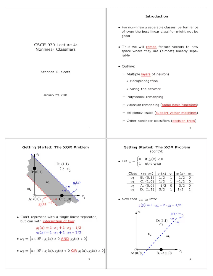Scott – Multiple layers of neurons ∗ Backpropagation ∗ Sizing the network January 29, 2001 – Polynomial remapping – Gaussian remapping (radial basis functions) – Efficiency issues (support vector machines) – Other nonlinear classifiers (decision trees) 1 2 Getting Started: The XOR Problem Getting Started: The XOR Problem (cont’d) x 2  0 if g i ( x ) < 0  • Let y i = 1 otherwise D: (1,1)  ω 2 B: (0,1) Class ( x 1 , x 2 ) g 1 ( x ) y 1 g 2 ( x ) y 2 ω 1 B: (0 , 1) 1 / 2 1 − 1 / 2 0 ω 1 ω 1 C: (1 , 0) 1 / 2 1 − 1 / 2 0 g (x) 2 ω 2 A: (0 , 0) − 1 / 2 0 − 3 / 2 0 > 0 ω 2 ω 2 D: (1 , 1) 3 / 2 1 1 / 2 1 < 0 x 1 A: (0,0) C: (1,0) • Now feed y 1 , y 2 into: > 0 < 0 g (x) g ( y ) = 1 · y 1 − 2 · y 2 − 1 / 2 1 y 2 g(y) • Can’t represent with a single linear separator, < 0 D: (1,1) but can with intersection of two: > 0 g 1 ( x ) = 1 · x 1 + 1 · x 2 − 1 / 2 g 2 ( x ) = 1 · x 1 + 1 · x 2 − 3 / 2 ω ω 1 2 � � x ∈ ℜ ℓ : g 1 ( x ) > 0 AND g 2 ( x ) < 0 • ω 1 = � � x ∈ ℜ ℓ : g 1 ( x ) , g 2 ( x ) < 0 OR g 1 ( x ) , g 2 ( x ) > 0 y • ω 2 = 1 A: (0,0) B, C: (1,0) 3 4

Getting Started: The XOR Problem What Else Can We Do with Two Layers? (cont’d) ω 2 > 0 g 3 111 • In other words, we remapped all vectors x to y < 0 ω such that the classes are linearly separable in 2 ω 110 = y y y the new vector space 011 1 1 2 3 ω 2 010 > 0 g ω ω < 0 2 2 w = -1/2 1 100 ω 001 Hidden Layer 01 1 y 1 > 0 000 < 0 g 1 w = -1/2 Σ w = 1 03 w x 11 w = 1 i1 i ω i 13 111 011 1 ω 2 x 1 Σ Input Layer w = 1 w y 21 i3 i i x w = 1 2 12 Σ w = -2 w = 1 Output w i2 x i 23 22 010 i 110 Layer ω y 2 2 ω 2 w = -3/2 02 ω 1 001 101 • This is a two-layer perceptron or two-layer unused feedforward neural network • Each neuron outputs 1 if its weighted sum ex- ω ceeds its threshold, 0 otherwise 1 ω 000 100 2 5 6 What Else Can We Do with Two Layers? Three-Layer Networks (cont’d) • With two-layer networks, there exist unions of • Define the p -dimensional unit hypercube as polyhedra not linearly separable on H p � � [ y 1 , . . . , y p ] T ∈ ℜ p , y i ∈ [0 , 1] ∀ i H p = • I.e. there exist assignments of classes to points on H p that are not linearly separable • A hidden layer with p neurons maps an ℓ -dim vector x to a p -dim vector y whose elements are corners of H p , i.e. y i ∈ { 0 , 1 } ∀ i • Solution: Add a second hidden layer of q neu- rons to partition H p into regions based on class • Each of the p neurons corresponds to an ℓ -dim hyperplane • Output layer combines appropriate regions • The intersection ∗ of the (pos. or neg.) half- • E.g. including 110 from Slide 6 in ω 1 is possible spaces from these p hyperplanes maps to a using procedure similar to XOR solution vertex of H p • If the classes of H p ’s vertices are linearly sep- • In general, can always use simple procedure arable, then a perfect two-layer network exists of isolating each ω 1 node in H p with its own second-layer hyperplane and taking disjunction • I.e. a 2-layer network can separate classes con- sisting of unions of adjacent polyhedra • Thus, can use 3-layer network to perfectly clas- sify any union polyhedral regions ∗ Also known as polyhedra. 7 8

The Backpropagation Algorithm The Backpropagation Algorithm • A popular way to train a neural network Nodes f f f Layer r • Assume the architecture is fixed and complete Σ Σ Σ r k · k r = number of nodes in layer r (could have Node j k L > 1) Node i r - 1 ji i r y w · w r ji = weight from neuron i in layer r − 1 to k r - 1 Nodes f f f Layer r - 1 neuron j in layer r Σ Σ Σ j = � k r − 1 jk y r − 1 · v r k =1 w r + w r k j 0 � � · y r v r j = f = output of neuron j in layer r j 1 1 1 1 1 k i y y y Nodes • During training we’ll attempt to minimize a f f f Layer 1 cost function, so use differentiable activation func. Σ Σ Σ k 1 f , e.g.: 1j 0 1 k k i1 w 1 1 w 1 1 w 1 ij w f ( v ) = 1 + e − av ∈ [0 , 1] Layer 0 (Input) 11 1 w Nodes 0 OR 1 k j x x x k 0 f ( v ) = c tanh ( av ) ∈ [ − c, c ] 9 10 The Backpropagation Algorithm Intuition The Backpropagation Algorithm Another Picture • Recall derivation of Perceptron update rule: – Cost function: ℓ � ( w i ( t + 1) − w i ( t )) 2 + U ( w ) = i =1 2   ℓ � η  y ( t ) − w i ( t + 1) x i ( t )  i =1 – Take gradient w.r.t. w ( t + 1), set to 0 , approximate, and solve: w i ( t + 1) = w i ( t ) +   ℓ �  x i ( t ) η  y ( t ) − w i ( t ) x i ( t ) i =1 11 12

The Backpropagation Algorithm The Backpropagation Algorithm Intuition: Output Layer Intuition: Output Layer (cont’d) • Now use similar idea with j th node of output layer (layer L ): • Again, approximate and solve for w L jk ( t + 1): – Cost function: k L − 1 � 2 + � � � � w L w L jk ( t + 1) − w L jk ( t ) + η y L − 1 w L jk ( t + 1) = w L U = jk ( t ) ( t ) · j k k =1       k L − 1 k L − 1 2   � jk ( t ) y L − 1 � jk ( t ) y L − 1 pred = y L w L  · f ′ w L j ( t ) with w ( t +1)  y j ( t ) − f   ( t )    ( t )   k   k    � �� �   k =1 k =1   correct k L − 1   � �� �  � jk ( t + 1) y L − 1  w L η y j ( t ) − f  ( t )     k     k =1    • So:   � � �� f ′ � � w L jk ( t + 1) = w L jk ( t ) + η y L − 1 v L v L ( t ) y j ( t ) − f j ( t ) j ( t ) – Take gradient w.r.t. w L k j ( t +1) and set to 0 : � �� � δ L j ( t )= “error term” � � w L jk ( t + 1) − w L 0 = 2 jk ( t )     k L − 1 � w L jk ( t + 1) y L − 1 • For f ( v ) = 1 / (1 + exp( − av )):     − 2 η  y j ( t ) − f ( t )  k   k =1 � � � � δ L j ( t ) = a · y L y j ( t ) − y L 1 − y L j ( t ) · j ( t ) j ( t )   k L − 1 � jk ( t + 1) y L − 1  y L − 1 · f ′ w L where y j ( t ) = target and y L  ( t )  ( t ) j ( t ) = output  k k k =1 13 14 The Backpropagation Algorithm The Backpropagation Algorithm Example Intuition: The Other Layers target = y trial 1: a = 1, b = 0, y = 1 • How can we compute the “error term” for the f(x) = 1 / (1 + exp(- x)) trial 2: a = 0, b = 1, y = 0 hidden layers r < L when there is no “target w a ca y c y d sum d vector” y for these layers? sum c c f d f w dc w cb b w d0 w c0 • Instead, propagate back error values from out- 1 1 put layer toward input layers, scaling with the weights eta 0.3 trial 1 trial 2 • Scaling with the weights characterizes how much w_ca 0.1 0.1008513 0.1008513 w_cb 0.1 0.1 0.0987985 of the error term each hidden unit is “respon- w_c0 0.1 0.1008513 0.0996498 sible for”: a 1 0 b 0 1 const 1 1 sum_c 0.2 0.2008513 w r jk ( t + 1) = w r jk ( t ) + η y r − 1 ( t ) δ r y_c 0.5498340 0.5500447 j ( t ) k w_dc 0.1 0.1189104 0.0964548 where w_d0 0.1 0.1343929 0.0935679 sum_d 0.1549834 0.1997990 � k r +1 j ( t ) = f ′ � y_d 0.5386685 0.5497842 � δ r +1 ( t ) w r +1 δ r v r j ( t ) ( t ) k kj target 1 0 k =1 delta_d 0.1146431 -0.136083 delta_c 0.0028376 -0.004005 • Derivation comes from computing gradient of cost function w.r.t. w r j ( t + 1) via chain rule delta_d(t) = y_d(t) * (y(t) - y_d(t)) * (1 - y_d(t)) delta_c(t) = y_c(t) * (1 - y_c(t)) * delta_d(t) * w_dc(t) w_dc(t+1) = w_dc(t) + eta * y_c(t) * delta_d(t) 15 w_ca(t+1) = w_ca(t) + eta * a * delta_c(t) 16

The Backpropagation Algorithm Issues • When to stop iterating through training set? The Backpropagation Algorithm – When weights don’t change much Issues (cont’d) – When value of cost function is small enough – Must also avoid overtraining • How to set learning rate η ( µ in text)? – Small values slow convergence – Large values might overshoot minimum – Can adapt it over time • Might hit local minima that aren’t very good; try re-running with new random weights 17 18 Variations • Can smooth oscillations of weight vector with momentum term α < 1 that tends to keep it Variations moving in the same direction as previous trials: (cont’d) ∆ w r j ( t + 1) = α ∆ w r j ( t ) + η y r − 1 ( t ) δ r j ( t ) k w r j ( t + 1) = w r j ( t ) + ∆ w r • A Recurrent network feeds output of e.g. layer j ( t + 1) r to the input of some earlier layer r ′ < r • Different training modes: – Allows predictions to be influenced by past predictions (for e.g. sequence data) – On-line (what we presented) has more ran- domness during training (might avoid local minima) – Batch mode (in text) averages gradients, giving better estimates and smoother con- vergence: ∗ Before updating, first compute δ r j ( t ) for each vector x t , t = 1 , . . . , N N � w r j (new) = w r δ r j ( t ) y r − 1 ( t ) j (old) + η t =1 19 20