CS70: Lecture 28. Review: Independence Variance Definition - - PowerPoint PPT Presentation

CS70: Lecture 28.

Variance; Inequalities; WLLN

• 1. Review: Independence
• 2. Variance
• 3. Inequalities

◮ Markov ◮ Chebyshev

• 4. Weak Law of Large Numbers

Review: Independence

Definition X and Y are independent ⇔ Pr[X = x,Y = y] = Pr[X = x]Pr[Y = y],∀x,y ⇔ Pr[X ∈ A,Y ∈ B] = Pr[X ∈ A]Pr[Y ∈ B],∀A,B. Theorem X and Y are independent ⇒ f(X),g(Y) are independent ∀f(·),g(·) ⇒ E[XY] = E[X]E[Y].

Variance

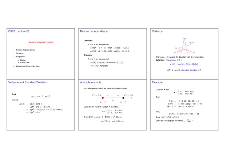
The variance measures the deviation from the mean value. Definition: The variance of X is σ2(X) := var[X] = E[(X −E[X])2]. σ(X) is called the standard deviation of X.

Variance and Standard Deviation

Fact: var[X] = E[X 2]−E[X]2. Indeed: var(X) = E[(X −E[X])2] = E[X 2 −2XE[X]+E[X]2) = E[X 2]−2E[X]E[X]+E[X]2, by linearity = E[X 2]−E[X]2.

A simple example

This example illustrates the term ‘standard deviation.’ Consider the random variable X such that X =

• µ −σ,

w.p. 1/2 µ +σ, w.p. 1/2. Then, E[X] = µ and (X −E[X])2 = σ2. Hence, var(X) = σ2 and σ(X) = σ.

Example

Consider X with X =

• −1,
• w. p. 0.99

99,

• w. p. 0.01.

Then E[X] = −1×0.99+99×0.01 = 0. E[X 2] = 1×0.99+(99)2 ×0.01 ≈ 100. Var(X) ≈ 100 = ⇒ σ(X) ≈ 10. Also, E(|X|) = 1×0.99+99×0.01 = 1.98. Thus, σ(X) = E[|X −E[X]|]! Exercise: How big can you make

σ(X) E[|X−E[X]|]?

Uniform

Assume that Pr[X = i] = 1/n for i ∈ {1,...,n}. Then E[X] =

n

∑

i=1

i ×Pr[X = i] = 1 n

n

∑

i=1

i = 1 n n(n +1) 2 = n +1 2 . Also, E[X 2] =

n

∑

i=1

i2Pr[X = i] = 1 n

n

∑

i=1

i2 = 1+3n +2n2 6 , as you can verify. This gives var(X) = 1+3n +2n2 6 − (n +1)2 4 = n2 −1 12 .

Variance of geometric distribution.

X is a geometrically distributed RV with parameter p. Thus, Pr[X = n] = (1−p)n−1p for n ≥ 1. Recall E[X] = 1/p. E[X 2] = p +4p(1−p)+9p(1−p)2 +... −(1−p)E[X 2] = −[p(1−p)+4p(1−p)2 +...] pE[X 2] = p +3p(1−p)+5p(1−p)2 +... = 2(p +2p(1−p)+3p(1−p)2 +..) E[X]! −(p +p(1−p)+p(1−p)2 +...) Distribution. pE[X 2] = 2E[X]−1 = 2(1 p)−1 = 2−p p = ⇒ E[X 2] = (2−p)/p2 and var[X] = E[X 2]−E[X]2 = 2−p

p2 − 1 p2 = 1−p p2 .

σ(X) = √

1−p p

≈ E[X] when p is small(ish).

Fixed points.

Number of fixed points in a random permutation of n items. “Number of student that get homework back.” X = X1 +X2 ···+Xn where Xi is indicator variable for ith student getting hw back. E(X 2) =

∑

i

E(X 2

i )+∑ i=j

E(XiXj). = n × 1 n +(n)(n −1)× 1 n(n −1) = 1+1 = 2. E(X 2

i ) = 1×Pr[Xi = 1]+0×Pr[Xi = 0]

= 1

n

E(XiXj) = 1×Pr[Xi = 1∩Xj = 1]+0×Pr[“anything else’′] = 1×1×(n−2)!

n!

=

1 n(n−1)

Var(X) = E(X 2)−(E(X))2 = 2−1 = 1.

Variance: binomial.

E[X 2] =

n

∑

i=0

i2 n i

• pi(1−p)n−i.

= Really???!!##... Too hard! Ok.. fine. Let’s do something else. Maybe not much easier...but there is a payoff.

Properties of variance.

• 1. Var(cX) = c2Var(X), where c is a constant.

Scales by c2.

• 2. Var(X +c) = Var(X), where c is a constant.

Shifts center. Proof: Var(cX) = E((cX)2)−(E(cX))2 = c2E(X 2)−c2(E(X))2 = c2(E(X 2)−E(X)2) = c2Var(X) Var(X +c) = E((X +c −E(X +c))2) = E((X +c −E(X)−c)2) = E((X −E(X))2) = Var(X)

Variance of sum of two independent random variables

Theorem: If X and Y are independent, then Var(X +Y) = Var(X)+Var(Y). Proof: Since shifting the random variables does not change their variance, let us subtract their means. That is, we assume that E(X) = 0 and E(Y) = 0. Then, by independence, E(XY) = E(X)E(Y) = 0. Hence, var(X +Y) = E((X +Y)2) = E(X 2 +2XY +Y 2) = E(X 2)+2E(XY)+E(Y 2) = E(X 2)+E(Y 2) = var(X)+var(Y).

Variance of sum of independent random variables

Theorem: If X,Y,Z,... are pairwise independent, then var(X +Y +Z +···) = var(X)+var(Y)+var(Z)+··· . Proof: Since shifting the random variables does not change their variance, let us subtract their means. That is, we assume that E[X] = E[Y] = ··· = 0. Then, by independence, E[XY] = E[X]E[Y] = 0. Also, E[XZ] = E[YZ] = ··· = 0. Hence, var(X +Y +Z +···) = E((X +Y +Z +···)2) = E(X 2 +Y 2 +Z 2 +···+2XY +2XZ +2YZ +···) = E(X 2)+E(Y 2)+E(Z 2)+···+0+···+0 = var(X)+var(Y)+var(Z)+··· .

Variance of Binomial Distribution.

Flip coin with heads probability p. X- how many heads? Xi =

• 1

if ith flip is heads

• therwise

E(X 2

i ) = 12 ×p +02 ×(1−p) = p.

Var(Xi) = p −(E(X))2 = p −p2 = p(1−p). p = 0 = ⇒ Var(Xi) = 0 p = 1 = ⇒ Var(Xi) = 0 X = X1 +X2 +...Xn. Xi and Xj are independent: Pr[Xi = 1|Xj = 1] = Pr[Xi = 1]. Var(X) = Var(X1 +···Xn) = np(1−p).

Inequalities: An Overview

n p n

µ P r [|X − µ | > ]

• Chebyshev

n p n

p n

Distribution

n p n

P r [X > a ] a Markov µ

Andrey Markov

Andrey Markov is best known for his work on stochastic processes. A primary subject of his research later became known as Markov chains and Markov processes. Pafnuty Chebyshev was one of his teachers. Markov was an atheist. In 1912 he protested Leo Tolstoy’s excommunication from the Russian Orthodox Church by requesting his

• wn excommunication. The Church complied

with his request.

Markov’s inequality

The inequality is named after Andrey Markov, although it appeared earlier in the work of Pafnuty Chebyshev. It should be (and is sometimes) called Chebyshev’s first inequality.

Theorem Markov’s Inequality Assume f : ℜ → [0,∞) is nondecreasing. Then, Pr[X ≥ a] ≤ E[f(X)] f(a) , for all a such that f(a) > 0. Proof: Observe that 1{X ≥ a} ≤ f(X) f(a) . Indeed, if X < a, the inequality reads 0 ≤ f(X)/f(a), which holds since f(·) ≥ 0. Also, if X ≥ a, it reads 1 ≤ f(X)/f(a), which holds since f(·) is nondecreasing. Taking the expectation yields the inequality, because expectation is monotone.

A picture

Markov Inequality Example: G(p)

Let X = G(p). Recall that E[X] = 1

p and E[X 2] = 2−p p2 .

Choosing f(x) = x, we get Pr[X ≥ a] ≤ E[X] a = 1 ap . Choosing f(x) = x2, we get Pr[X ≥ a] ≤ E[X 2] a2 = 2−p p2a2 .

Markov Inequality Example: P(λ)

Let X = P(λ). Recall that E[X] = λ and E[X 2] = λ +λ 2. Choosing f(x) = x, we get Pr[X ≥ a] ≤ E[X] a = λ a . Choosing f(x) = x2, we get Pr[X ≥ a] ≤ E[X 2] a2 = λ +λ 2 a2 .

Chebyshev’s Inequality

This is Pafnuty’s inequality: Theorem: Pr[|X −E[X]| > a] ≤ var[X] a2 , for all a > 0. Proof: Let Y = |X −E[X]| and f(y) = y2. Then, Pr[Y ≥ a] ≤ E[f(Y)] f(a) = var[X] a2 . This result confirms that the variance measures the “deviations from the mean.”

Chebyshev and Poisson

Let X = P(λ). Then, E[X] = λ and var[X] = λ. Thus, Pr[|X −λ| ≥ n] ≤ var[X] n2 = λ n2 .

Chebyshev and Poisson (continued)

Let X = P(λ). Then, E[X] = λ and var[X] = λ. By Markov’s inequality, Pr[X ≥ a] ≤ E[X 2] a2 = λ +λ 2 a2 . Also, if a > λ, then X ≥ a ⇒ X −λ ≥ a−λ > 0 ⇒ |X −λ| ≥ a−λ. Hence, for a > λ, Pr[X ≥ a] ≤ Pr[|X −λ| ≥ a−λ] ≤

λ (a−λ)2 .

Fraction of H’s

Here is a classical application of Chebyshev’s inequality. How likely is it that the fraction of H’s differs from 50%? Let Xm = 1 if the m-th flip of a fair coin is H and Xm = 0 otherwise. Define Yn = X1 +···+Xn n , for n ≥ 1. We want to estimate Pr[|Yn −0.5| ≥ 0.1] = Pr[Yn ≤ 0.4 or Yn ≥ 0.6]. By Chebyshev, Pr[|Yn −0.5| ≥ 0.1] ≤ var[Yn]

(0.1)2 = 100var[Yn].

Now, var[Yn] = 1

n2 (var[X1]+···+var[Xn]) = 1 nvar[X1] ≤ 1 4n.

Var(Xi) = p(1−lp) ≤ (.5)(.5) = 1

4

Fraction of H’s

Yn = X1 +···+Xn n , for n ≥ 1. Pr[|Yn −0.5| ≥ 0.1] ≤ 25 n . For n = 1,000, we find that this probability is less than 2.5%. As n → ∞, this probability goes to zero. In fact, for any ε > 0, as n → ∞, the probability that the fraction of Hs is within ε > 0 of 50% approaches 1: Pr[|Yn −0.5| ≤ ε] → 1. This is an example of the Law of Large Numbers. We look at a general case next.

Weak Law of Large Numbers

Theorem Weak Law of Large Numbers Let X1,X2,... be pairwise independent with the same distribution and mean µ. Then, for all ε > 0, Pr[|X1 +···+Xn n − µ| ≥ ε] → 0, as n → ∞. Proof: Let Yn = X1+···+Xn

n

. Then Pr[|Yn − µ| ≥ ε] ≤ var[Yn] ε2 = var[X1 +···+Xn] n2ε2 = nvar[X1] n2ε2 = var[X1] nε2 → 0, as n → ∞.

Summary

Variance; Inequalities; WLLN

◮ Variance: var[X] := E[(X −E[X])2] = E[X 2]−E[X]2 ◮ Fact: var[aX +b]a2var[X] ◮ Sum: X,Y,Z pairwise ind. ⇒ var[X +Y +Z] = ··· ◮ Markov: Pr[X ≥ a] ≤ E[f(X)]/f(a) where ... ◮ Chebyshev: Pr[|X −E[X]| ≥ a] ≤ var[X]/a2 ◮ WLLN: Xm i.i.d. ⇒ X1+···+Xn n

≈ E[X]