CS70: Lecture 20. Review: Expectation Uniform Distribution - - PowerPoint PPT Presentation

CS70: Lecture 20.

Distributions; Independent RVs

• 1. Review: Expectation
• 2. Distributions
• 3. Independent RVs

Review: Expectation

◮ E[X] := ∑x xPr[X = x] = ∑ω X(ω)Pr[ω]. ◮ E[g(X,Y)] = ∑x,y g(x,y)Pr[X = x,Y = y]

= ∑ω g(X(ω),Y(ω))Pr[ω]

◮ E[aX +bY +c] = aE[X]+bE[Y]+c.

Uniform Distribution

Roll a six-sided balanced die. Let X be the number of pips (dots). Then X is equally likely to take any of the values {1,2,...,6}. We say that X is uniformly distributed in {1,2,...,6}. More generally, we say that X is uniformly distributed in {1,2,...,n} if Pr[X = m] = 1/n for m = 1,2,...,n. In that case, E[X] =

n

∑

m=1

mPr[X = m] =

n

∑

m=1

m × 1 n = 1 n n(n +1) 2 = n +1 2 .

Geometric Distribution

Let’s flip a coin with Pr[H] = p until we get H. For instance: ω1 = H, or ω2 = T H, or ω3 = T T H, or ωn = T T T T ··· T H. Note that Ω = {ωn,n = 1,2,...}. Let X be the number of flips until the first H. Then, X(ωn) = n. Also, Pr[X = n] = (1−p)n−1p, n ≥ 1.

Geometric Distribution

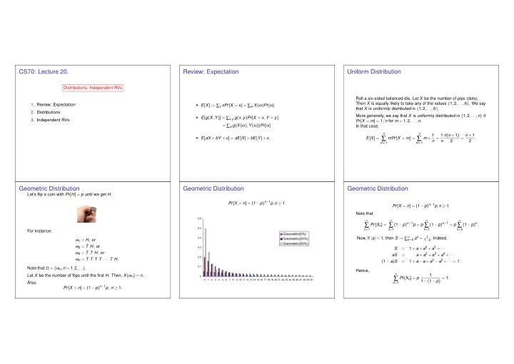
Pr[X = n] = (1−p)n−1p,n ≥ 1.

Geometric Distribution

Pr[X = n] = (1−p)n−1p,n ≥ 1. Note that

∞

∑

n=1

Pr[Xn] =

∞

∑

n=1

(1−p)n−1p = p

∞

∑

n=1

(1−p)n−1 = p

∞

∑

n=0

(1−p)n. Now, if |a| < 1, then S := ∑∞

n=0 an = 1 1−a. Indeed,

S = 1+a+a2 +a3 +··· aS = a+a2 +a3 +a4 +··· (1−a)S = 1+a−a+a2 −a2 +··· = 1. Hence,

∞

∑

n=1

Pr[Xn] = p 1 1−(1−p) = 1.

Geometric Distribution: Expectation

X =D G(p), i.e., Pr[X = n] = (1−p)n−1p,n ≥ 1. One has E[X] =

∞

∑

n=1

nPr[X = n] =

∞

∑

n=1

n(1−p)n−1p. Thus, E[X] = p +2(1−p)p +3(1−p)2p +4(1−p)3p +··· (1−p)E[X] = (1−p)p +2(1−p)2p +3(1−p)3p +··· pE[X] = p + (1−p)p + (1−p)2p + (1−p)3p +··· by subtracting the previous two identities =

∞

∑

n=1

Pr[X = n] = 1. Hence, E[X] = 1 p.

Coupon Collectors Problem.

Experiment: Get coupons at random from n until collect all n coupons. Outcomes: {123145...,56765...} Random Variable: X - length of outcome. Before: Pr[X ≥ nln2n] ≤ 1

2.

Today: E[X]?

Time to collect coupons

X-time to get n coupons. X1 - time to get first coupon. Note: X1 = 1. E(X1) = 1. X2 - time to get second coupon after getting first. Pr[“get second coupon”|“got milk —- first coupon”] = n−1

n

E[X2]? Geometric ! ! ! = ⇒ E[X2] = 1

p = 1

n−1 n

=

n n−1.

Pr[“getting ith coupon|“got i −1rst coupons”] = n−(i−1)

n

= n−i+1

n

E[Xi] = 1

p = n n−i+1,i = 1,2,...,n.

E[X] = E[X1]+···+E[Xn] = n n + n n −1 + n n −2 +···+ n 1 = n(1+ 1 2 +···+ 1 n) =: nH(n) ≈ n(lnn +γ)

Review: Harmonic sum

H(n) = 1+ 1 2 +···+ 1 n ≈

n

1

1 x dx = ln(n). . A good approximation is H(n) ≈ ln(n)+γ where γ ≈ 0.58 (Euler-Mascheroni constant).

Harmonic sum: Paradox

Consider this stack of cards (no glue!): If each card has length 2, the stack can extend H(n) to the right of the

• table. As n increases, you can go as far as you want!

Paradox

Stacking

The cards have width 2. Induction shows that the center of gravity after n cards is H(n) away from the right-most edge.

Geometric Distribution: Memoryless

Let X be G(p). Then, for n ≥ 0, Pr[X > n] = Pr[ first n flips are T] = (1−p)n. Theorem Pr[X > n +m|X > n] = Pr[X > m],m,n ≥ 0. Proof: Pr[X > n +m|X > n] = Pr[X > n +m and X > n] Pr[X > n] = Pr[X > n +m] Pr[X > n] = (1−p)n+m (1−p)n = (1−p)m = Pr[X > m].

Geometric Distribution: Memoryless - Interpretation

Pr[X > n +m|X > n] = Pr[X > m],m,n ≥ 0. Pr[X > n +m|X > n] = Pr[A|B] = Pr[A] = Pr[X > m]. The coin is memoryless, therefore, so is X.

Geometric Distribution: Yet another look

Theorem: For a r.v. X that takes the values {0,1,2,...}, one has E[X] =

∞

∑

i=1

Pr[X ≥ i]. [See later for a proof.] If X = G(p), then Pr[X ≥ i] = Pr[X > i −1] = (1−p)i−1. Hence, E[X] =

∞

∑

i=1

(1−p)i−1 =

∞

∑

i=0

(1−p)i = 1 1−(1−p) = 1 p.

Expected Value of Integer RV

Theorem: For a r.v. X that takes values in {0,1,2,...}, one has E[X] =

∞

∑

i=1

Pr[X ≥ i]. Proof: One has E[X] =

∞

∑

i=1

i ×Pr[X = i] =

∞

∑

i=1

i{Pr[X ≥ i]−Pr[X ≥ i +1]} =

∞

∑

i=1

{i ×Pr[X ≥ i]−i ×Pr[X ≥ i +1]} =

∞

∑

i=1

{i ×Pr[X ≥ i]−(i −1)×Pr[X ≥ i]} =

∞

∑

i=1

Pr[X ≥ i]. Theorem: For a r.v. X that takes values in {0,1,2,...}, one has E[X] =

∞

∑

i=1

Pr[X ≥ i]. 1 2 3 ··· Pr[X ≥ 1] Pr[X ≥ 2] Pr[X ≥ 3] . . . Probability mass at i, counted i times. Same as ∑∞

i=1 i ×Pr[X = i].

Poisson

Experiment: flip a coin n times. The coin is such that Pr[H] = λ/n. Random Variable: X - number of heads. Thus, X = B(n,λ/n). Poisson Distribution is distribution of X “for large n.”

Poisson

Experiment: flip a coin n times. The coin is such that Pr[H] = λ/n. Random Variable: X - number of heads. Thus, X = B(n,λ/n). Poisson Distribution is distribution of X “for large n.” We expect X ≪ n. For m ≪ n one has Pr[X = m] = n m

• pm(1−p)n−m, with p = λ/n

= n(n −1)···(n −m +1) m! λ n m 1− λ n n−m = n(n −1)···(n −m +1) nm λ m m!

• 1− λ

n n−m ≈(1) λ m m!

• 1− λ

n n−m ≈(2) λ m m!

• 1− λ

n n ≈ λ m m! e−λ. For (1) we used m ≪ n; for (2) we used (1−a/n)n ≈ e−a.

Poisson Distribution: Definition and Mean

Definition Poisson Distribution with parameter λ > 0 X = P(λ) ⇔ Pr[X = m] = λ m m! e−λ,m ≥ 0. Fact: E[X] = λ. Proof: E[X] =

∞

∑

m=1

m × λ m m! e−λ = e−λ

∞

∑

m=1

λ m (m −1)! = e−λ

∞

∑

m=0

λ m+1 m! = e−λλ

∞

∑

m=0

λ m m! = e−λλeλ = λ.

Simeon Poisson

The Poisson distribution is named after:

Equal Time: B. Geometric

The geometric distribution is named after:

• Prof. Walrand could not find a picture of D. Binomial, sorry.

Review: Distributions

◮ U[1,...,n] : Pr[X = m] = 1 n,m = 1,...,n;

E[X] = n+1

2 ; ◮ B(n,p) : Pr[X = m] =

n

m

• pm(1−p)n−m,m = 0,...,n;

E[X] = np;

◮ G(p) : Pr[X = n] = (1−p)n−1p,n = 1,2,...;

E[X] = 1

p; ◮ P(λ) : Pr[X = n] = λ n n! e−λ,n ≥ 0;

E[X] = λ.

Independent Random Variables.

Definition: Independence The random variables X and Y are independent if and only if Pr[Y = b|X = a] = Pr[Y = b], for all a and b. Fact: X,Y are independent if and only if Pr[X = a,Y = b] = Pr[X = a]Pr[Y = b], for all a and b. Obvious.

Independence: Examples

Example 1 Roll two die. X,Y = number of pips on the two dice. X,Y are independent. Indeed: Pr[X = a,Y = b] = 1

36,Pr[X = a] = Pr[Y = b] = 1 6.

Example 2 Roll two die. X = total number of pips, Y = number of pips on die 1 minus number on die 2. X and Y are not independent. Indeed: Pr[X = 12,Y = 1] = 0 = Pr[X = 12]Pr[Y = 1] > 0. Example 3 Flip a fair coin five times, X = number of Hs in first three flips, Y = number of Hs in last two flips. X and Y are independent. Indeed: Pr[X = a,Y = b] = 3 a 2 b

• 2−5 =

3 a

• 2−3×

2 b

• 2−2 = Pr[X = a]Pr[Y = b].

A useful observation about independence

Theorem X and Y are independent if and only if Pr[X ∈ A,Y ∈ B] = Pr[X ∈ A]Pr[Y ∈ B] for all A,B ⊂ ℜ. Proof: If (⇐): Choose A = {a} and B = {b}. This shows that Pr[X = a,Y = b] = Pr[X = a]Pr[Y = b]. Only if (⇒): Pr[X ∈ A,Y ∈ B] = ∑

a∈A ∑ b∈B

Pr[X = a,Y = b] = ∑

a∈A ∑ b∈B

Pr[X = a]Pr[Y = b] = ∑

a∈A

[∑

b∈B

Pr[X = a]Pr[Y = b]] = ∑

a∈A

Pr[X = a][∑

b∈B

Pr[Y = b]] = ∑

a∈A

Pr[X = a]Pr[Y ∈ B] = Pr[X ∈ A]Pr[Y ∈ B].

Functions of Independent random Variables

Theorem Functions of independent RVs are independent Let X,Y be independent RV. Then f(X) and g(Y) are independent, for all f(·),g(·). Proof: Recall the definition of inverse image: h(z) ∈ C ⇔ z ∈ h−1(C) := {z | h(z) ∈ C}. (1) Now, Pr[f(X) ∈ A,g(Y) ∈ B] = Pr[X ∈ f −1(A),Y ∈ g−1(B)], by (1) = Pr[X ∈ f −1(A)]Pr[Y ∈ g−1(B)], since X,Y ind. = Pr[f(X) ∈ A]Pr[g(Y) ∈ B], by (1).

Mean of product of independent RV

Theorem Let X,Y be independent RVs. Then E[XY] = E[X]E[Y]. Proof: Recall that E[g(X,Y)] = ∑x,y g(x,y)Pr[X = x,Y = y]. Hence, E[XY] = ∑

x,y

xyPr[X = x,Y = y] = ∑

x,y

xyPr[X = x]Pr[Y = y], by ind. = ∑

x

[∑

y

xyPr[X = x]Pr[Y = y]] = ∑

x

[xPr[X = x](∑

y

yPr[Y = y])] = ∑

x

[xPr[X = x]E[Y]] = E[X]E[Y].

Examples

(1) Assume that X,Y,Z are (pairwise) independent, with E[X] = E[Y] = E[Z] = 0 and E[X 2] = E[Y 2] = E[Z 2] = 1. Then E[(X +2Y +3Z)2] = E[X 2 +4Y 2 +9Z 2 +4XY +12YZ +6XZ] = 1+4+9+4×0+12×0+6×0 = 14. (2) Let X,Y be independent and U[1,2,...n]. Then E[(X −Y)2] = E[X 2 +Y 2 −2XY] = 2E[X 2]−2E[X]2 = 1+3n +2n2 3 − (n +1)2 2 .

Mutually Independent Random Variables

Definition X,Y,Z are mutually independent if Pr[X = x,Y = y,Z = z] = Pr[X = x]Pr[Y = y]Pr[Z = z], for all x,y,z. Theorem The events A,B,C,... are pairwise (resp. mutually) independent iff the random variables 1A,1B,1C,... are pairwise (resp. mutually) independent. Proof: Pr[1A = 1,1B = 1,1C = 1] = Pr[A∩B ∩C],...

Functions of pairwise independent RVs

If X,Y,Z are pairwise independent, but not mutually independent, it may be that f(X) and g(Y,Z) are not independent. Example 1: Flip two fair coins, X = 1{coin 1 is H},Y = 1{coin 2 is H},Z = X ⊕Y. Then, X,Y,Z are pairwise independent. Let g(Y,Z) = Y ⊕Z. Then g(Y,Z) = X is not independent of X. Example 2: Let A,B,C be pairwise but not mutually independent in a way that A and B ∩C are not independent. Let X = 1A,Y = 1B,Z = 1C. Choose f(X) = X,g(Y,Z) = YZ.

Functions of mutually independent RVs

One has the following result: Theorem Functions of disjoint collections of mutually independent random variables are mutually independent. Example: Let {Xn,n ≥ 1} be mutually independent. Then,

Y1 := X1X2(X3+X4)2,Y2 := max{X5,X6}−min{X7,X8},Y3 := X9 cos(X10+X11)

are mutually independent. Proof: Let B1 := {(x1,x2,x3,x4) | x1x2(x3 +x4)2 ∈ A1}. Similarly for B2,B2. Then Pr[Y1 ∈ A1,Y2 ∈ A2,Y3 ∈ A3] = Pr[(X1,...,X4) ∈ B1,(X5,...,X8) ∈ B2,(X9,...,X11) ∈ B3] = Pr[(X1,...,X4) ∈ B1]Pr[(X5,...,X8) ∈ B2]Pr[(X9,...,X11) ∈ B3] = Pr[Y1 ∈ A1]Pr[Y2 ∈ A2]Pr[Y3 ∈ A3]

Operations on Mutually Independent Events

Theorem Operations on disjoint collections of mutually independent events produce mutually independent events. For instance, if A,B,C,D,E are mutually independent, then A∆B,C \D, ¯ E are mutually independent. Proof: 1A∆B = f(1A,1B) where f(0,0) = 0,f(1,0) = 1,f(0,1) = 1,f(1,1) = 0 1C\D = g(1C,1D) where g(0,0) = 0,g(1,0) = 1,g(0,1) = 0,g(1,1) = 0 1¯

E = h(1E) where

h(0) = 1 and h(1) = 0. Hence, 1A∆B,1C\D,1¯

E are functions of mutually independent RVs.

Thus, those RVs are mutually independent. Consequently, the events

• f which they are indicators are mutually independent.

Product of mutually independent RVs

Theorem Let X1,...,Xn be mutually independent RVs. Then, E[X1X2 ···Xn] = E[X1]E[X2]···E[Xn]. Proof: Assume that the result is true for n. (It is true for n = 2.) Then, with Y = X1 ···Xn, one has E[X1 ···XnXn+1] = E[YXn+1], = E[Y]E[Xn+1], because Y,Xn+1 are independent = E[X1]···E[Xn]E[Xn+1].

Summary.

Distributions; Independence Distributions:

◮ G(p) : E[X] = 1/p; ◮ B(n,p) : E[X] = np; ◮ P(λ) : E[X] = λ

Independence:

◮ X,Y independent ⇔ Pr[X ∈ A,Y ∈ B] = Pr[X ∈ A]Pr[Y ∈ B] ◮ Then, f(X),g(Y) are independent

and E[XY] = E[X]E[Y]

◮ Mutual independence ....