CS70: Jean Walrand: Lecture 30. Linear Regression: Preamble Linear - PowerPoint PPT Presentation

X Y CS70: Jean Walrand: Lecture 30. Linear Regression: Preamble Linear Regression: Preamble Thus, if we want to guess the value of Y , we choose E [ Y ] . The best guess about Y , if we know only the distribution of Y , is E [ Y ] . Now assume we make some observation X related to Y . Linear Regression More precisely, the value of a that minimizes E [( Y − a ) 2 ] is a = E [ Y ] . How do we use that observation to improve our guess about Y ? Proof: Let ˆ Y := Y − E [ Y ] . Then, E [ ˆ Y ] = 0. So, E [ ˆ The idea is to use a function g ( X ) of the observation to 1. Preamble Yc ] = 0 , ∀ c . Now, estimate Y . 2. Motivation for LR E [( Y − a ) 2 ] E [( Y − E [ Y ]+ E [ Y ] − a ) 2 ] = The simplest function g ( X ) is a constant that does not depend 3. History of LR E [( ˆ Y + c ) 2 ] with c = E [ Y ] − a = of X . 4. Linear Regression Y 2 + 2 ˆ E [ ˆ Yc + c 2 ] = E [ ˆ Y 2 ]+ 2 E [ ˆ Yc ]+ c 2 = The next simplest function is linear: g ( X ) = a + bX . Y 2 ]+ 0 + c 2 ≥ E [ ˆ 5. Derivation E [ ˆ Y 2 ] . = What is the best linear function? That is our next topic. 6. More examples Hence, E [( Y − a ) 2 ] ≥ E [( Y − E [ Y ]) 2 ] , ∀ a . A bit later, we will consider a general function g ( X ) . 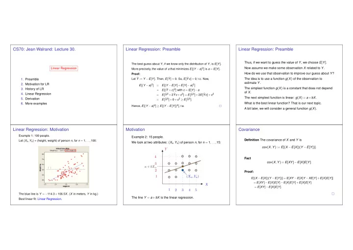Linear Regression: Motivation Motivation Covariance Example 1: 100 people. Example 2: 15 people. Definition The covariance of X and Y is Let ( X n , Y n ) = (height, weight) of person n , for n = 1 ,..., 100: We look at two attributes: ( X n , Y n ) of person n , for n = 1 ,..., 15: cov ( X , Y ) := E [( X − E [ X ])( Y − E [ Y ])] . Fact cov ( X , Y ) = E [ XY ] − E [ X ] E [ Y ] . E [ Y ] Proof: E [( X − E [ X ])( Y − E [ Y ])] = E [ XY − E [ X ] Y − XE [ Y ]+ E [ X ] E [ Y ]] = E [ XY ] − E [ X ] E [ Y ] − E [ X ] E [ Y ]+ E [ X ] E [ Y ] = E [ XY ] − E [ X ] E [ Y ] . The blue line is Y = − 114 . 3 + 106 . 5 X . ( X in meters, Y in kg.) The line Y = a + bX is the linear regression. Best linear fit: Linear Regression.

Examples of Covariance Examples of Covariance Properties of Covariance cov ( X , Y ) = E [( X − E [ X ])( Y − E [ Y ])] = E [ XY ] − E [ X ] E [ Y ] . Fact (a) var [ X ] = cov ( X , X ) (b) X , Y independent ⇒ cov ( X , Y ) = 0 (c) cov ( a + X , b + Y ) = cov ( X , Y ) (d) cov ( aX + bY , cU + dV ) = ac . cov ( X , U )+ ad . cov ( X , V ) + bc . cov ( Y , U )+ bd . cov ( Y , V ) . Proof: E [ X ] = 1 × 0 . 15 + 2 × 0 . 4 + 3 × 0 . 45 = 1 . 9 Note that E [ X ] = 0 and E [ Y ] = 0 in these examples. Then (a)-(b)-(c) are obvious. E [ X 2 ] = 1 2 × 0 . 15 + 2 2 × 0 . 4 + 3 2 × 0 . 45 = 5 . 8 cov ( X , Y ) = E [ XY ] . (d) In view of (c), one can subtract the means and assume that the RVs are zero-mean. Then, When cov ( X , Y ) > 0, the RVs X and Y tend to be large or small E [ Y ] = 1 × 0 . 2 + 2 × 0 . 6 + 3 × 0 . 2 = 2 together. X and Y are said to be positively correlated. cov ( aX + bY , cU + dV ) = E [( aX + bY )( cU + dV )] E [ XY ] = 1 × 0 . 05 + 1 × 2 × 0 . 1 + ··· + 3 × 3 × 0 . 2 = 4 . 85 = ac . E [ XU ]+ ad . E [ XV ]+ bc . E [ YU ]+ bd . E [ YV ] When cov ( X , Y ) < 0, when X is larger, Y tends to be smaller. X and cov ( X , Y ) = E [ XY ] − E [ X ] E [ Y ] = 1 . 05 Y are said to be negatively correlated. var [ X ] = E [ X 2 ] − E [ X ] 2 = 2 . 19 . = ac . cov ( X , U )+ ad . cov ( X , V )+ bc . cov ( Y , U )+ bd . cov ( Y , V ) . When cov ( X , Y ) = 0, we say that X and Y are uncorrelated. Linear Regression: Non-Bayesian Linear Least Squares Estimate LR: Non-Bayesian or Uniform? Definition Definition Given the samples { ( X n , Y n ) , n = 1 ,..., N } , the Linear Observe that Given two RVs X and Y with known distribution Regression of Y over X is Pr [ X = x , Y = y ] , the Linear Least Squares Estimate of Y given N 1 ( Y n − a − bX n ) 2 = E [( Y − a − bX ) 2 ] ∑ ˆ X is Y = a + bX N ˆ n = 1 Y = a + bX =: L [ Y | X ] where ( a , b ) minimize where one assumes that where ( a , b ) minimize N ( X , Y ) = ( X n , Y n ) , w.p. 1 g ( a , b ) := E [( Y − a − bX ) 2 ] . ( Y n − a − bX n ) 2 . N for n = 1 ,..., N . ∑ n = 1 Thus, ˆ Y = a + bX is our guess about Y given X . The squared That is, the non-Bayesian LR is equivalent to the Bayesian Thus, ˆ error is ( Y − ˆ Y ) 2 . The LLSE minimizes the expected value of Y n = a + bX n is our guess about Y n given X n . The LLSE that assumes that ( X , Y ) is uniform on the set of squared error is ( Y n − ˆ Y n ) 2 . The LR minimizes the sum of the the squared error. observed samples. squared errors. Why the squares and not the absolute values? Main Thus, we can study the two cases LR and LLSE in one shot. Why the squares and not the absolute values? Main justification: much easier! However, the interpretations are different! justification: much easier! Note: This is a Bayesian formulation: there is a prior. Note: This is a non-Bayesian formulation: there is no prior.

LLSE A Bit of Algebra Estimation Error Theorem Y − ˆ Y = ( Y − E [ Y ]) − cov ( X , Y ) var [ X ] ( X − E [ X ]) . We saw that the LLSE of Y given X is Consider two RVs X , Y with a given distribution Hence, E [ Y − ˆ Y ] = 0. We want to show that E [( Y − ˆ Pr [ X = x , Y = y ] . Then, Y ) X ] = 0. Y = E [ Y ]+ cov ( X , Y ) Y = E [ Y ]+ cov ( X , Y ) L [ Y | X ] = ˆ ( X − E [ X ]) . L [ Y | X ] = ˆ var ( X ) ( X − E [ X ]) . Note that var ( X ) E [( Y − ˆ Y ) X ] = E [( Y − ˆ Proof 1: Y )( X − E [ X ])] , Y − ˆ Y = ( Y − E [ Y ]) − cov ( X , Y ) var [ X ] ( X − E [ X ]) . Hence, E [ Y − ˆ How good is this estimator? That is, what is the mean squared Y ] = 0. because E [( Y − ˆ Y ) E [ X ]] = 0. estimation error? Also, E [( Y − ˆ Y ) X ] = 0 , after a bit of algebra. (See next slide.) Now, We find Hence, by combining the two brown equalities, E [( Y − ˆ E [ | Y − L [ Y | X ] | 2 ] = E [( Y − E [ Y ] − ( cov ( X , Y ) / var ( X ))( X − E [ X ])) 2 ] Y )( X − E [ X ])] E [( Y − ˆ Y )( c + dX )] = 0 . Then, E [( Y − ˆ Y )( ˆ Y − a − bX )] = 0 , ∀ a , b . = E [( Y − E [ Y ]) 2 ] − 2 ( cov ( X , Y ) / var ( X )) E [( Y − E [ Y ])( X − E [ X ])] Indeed: ˆ Y = α + β X for some α , β , so that ˆ = E [( Y − E [ Y ])( X − E [ X ])] − cov ( X , Y ) Y − a − bX = c + dX for E [( X − E [ X ])( X − E [ X ])] +( cov ( X , Y ) / var ( X )) 2 E [( X − E [ X ]) 2 ] var [ X ] some c , d . Now, = ( ∗ ) cov ( X , Y ) − cov ( X , Y ) = var ( Y ) − cov ( X , Y ) 2 E [( Y − a − bX ) 2 ] = E [( Y − ˆ Y + ˆ Y − a − bX ) 2 ] var [ X ] = 0 . . var ( X ) var [ X ] = E [( Y − ˆ Y ) 2 ]+ E [( ˆ Y − a − bX ) 2 ]+ 0 ≥ E [( Y − ˆ Y ) 2 ] . Without observations, the estimate is E [ Y ] = 0. The error is var ( Y ) . ( ∗ ) Recall that cov ( X , Y ) = E [( X − E [ X ])( Y − E [ Y ])] and Observing X reduces the error. This shows that E [( Y − ˆ Y ) 2 ] ≤ E [( Y − a − bX ) 2 ] , for all ( a , b ) . var [ X ] = E [( X − E [ X ]) 2 ] . Thus ˆ Y is the LLSE. Estimation Error: A Picture Linear Regression Examples Linear Regression Examples We saw that Example 2: Y = E [ Y ]+ cov ( X , Y ) L [ Y | X ] = ˆ Example 1: ( X − E [ X ]) var ( X ) and E [ | Y − L [ Y | X ] | 2 ] = var ( Y ) − cov ( X , Y ) 2 . var ( X ) Here is a picture when E [ X ] = 0 , E [ Y ] = 0: We find: E [ X ] = 0 ; E [ Y ] = 0 ; E [ X 2 ] = 1 / 2 ; E [ XY ] = 1 / 2 ; var [ X ] = E [ X 2 ] − E [ X ] 2 = 1 / 2 ; cov ( X , Y ) = E [ XY ] − E [ X ] E [ Y ] = 1 / 2 ; Y = E [ Y ]+ cov ( X , Y ) LR: ˆ ( X − E [ X ]) = X . var [ X ]

Linear Regression Examples Linear Regression Examples LR: Another Figure Example 4: Example 3: We find: We find: E [ X ] = 0 ; E [ Y ] = 0 ; E [ X 2 ] = 1 / 2 ; E [ XY ] = − 1 / 2 ; E [ X ] = 3 ; E [ Y ] = 2 . 5 ; E [ X 2 ] = ( 3 / 15 )( 1 + 2 2 + 3 2 + 4 2 + 5 2 ) = 11 ; Note that var [ X ] = E [ X 2 ] − E [ X ] 2 = 1 / 2 ; cov ( X , Y ) = E [ XY ] − E [ X ] E [ Y ] = − 1 / 2 ; E [ XY ] = ( 1 / 15 )( 1 × 1 + 1 × 2 + ··· + 5 × 4 ) = 8 . 4 ; ◮ the LR line goes through ( E [ X ] , E [ Y ]) Y = E [ Y ]+ cov ( X , Y ) LR: ˆ ( X − E [ X ]) = − X . var [ X ] = 11 − 9 = 2 ; cov ( X , Y ) = 8 . 4 − 3 × 2 . 5 = 0 . 9 ; var [ X ] ◮ its slope is cov ( X , Y ) var ( X ) . Y = 2 . 5 + 0 . 9 LR: ˆ 2 ( X − 3 ) = 1 . 15 + 0 . 45 X . Summary Linear Regression 1. Linear Regression: L [ Y | X ] = E [ Y ]+ cov ( X , Y ) var ( X ) ( X − E [ X ]) 2. Non-Bayesian: minimize ∑ n ( Y n − a − bX n ) 2 3. Bayesian: minimize E [( Y − a − bX ) 2 ]