CS4405 JPEG Transform Coding JPEG Compression Workflow RGB - - PowerPoint PPT Presentation

SLIDE 1

CS4405

JPEG Transform Coding

JPEG ¡Compression ¡Workflow

RGB YCbCr

Optional Chroma Subsample

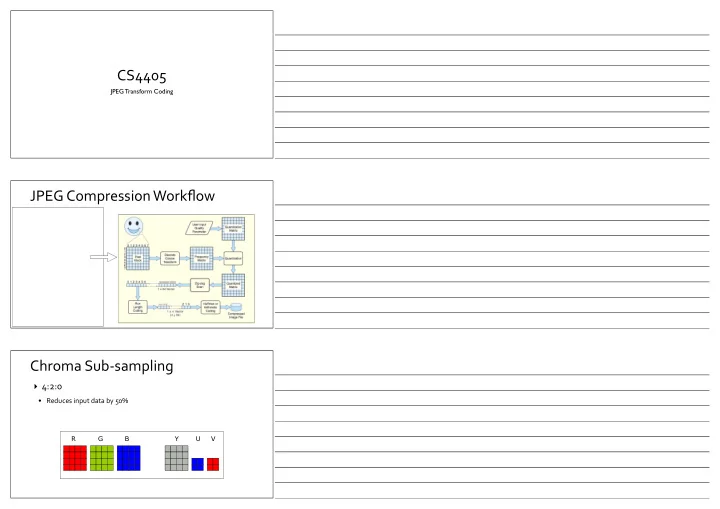
Chroma ¡Sub-­‑sampling

• 4:2:0
• Reduces ¡input ¡data ¡by ¡50%

R G B Y U V

SLIDE 2

Chroma ¡Sub-­‑sampling

luminance ¡

RGB ¡Components YCbCr ¡Components

More ¡resolution ¡in ¡Y ¡than ¡in ¡Cb ¡or ¡Cr

SLIDE 3

JPEG ¡Cb JPEG ¡Cr

YCb ¡Cr ¡After ¡JPEG ¡(Q=30%)

JPEG ¡Y

Simple ¡Example ¡Transform

• In ¡image ¡compression ¡the ¡data ¡is ¡usually ¡a ¡two-­‑

dimensional ¡array ¡of ¡pixels

• Typically ¡a ¡4x4 ¡8x8 ¡or ¡16x16 ¡block ¡of ¡pixels

A D C B Transform Inverse ¡Transform X0 ¡= ¡A X1 ¡= ¡B ¡-­‑ ¡A X2 ¡= ¡C ¡-­‑ ¡A X3 ¡= ¡D ¡-­‑ ¡A A ¡= ¡X0 D ¡= ¡X3 ¡+ ¡X0 C ¡= ¡X2 ¡+ ¡X0 B ¡= ¡X1 ¡+ ¡X0

Example ¡Transform

• If ¡the ¡pixels ¡were ¡8 ¡bits ¡each ¡then ¡the ¡block ¡would ¡use ¡32 ¡bits
• Using ¡the ¡transform ¡we ¡could ¡assign ¡4 ¡bits ¡each ¡for ¡the ¡difference ¡values ¡and ¡8 ¡

bits ¡for ¡the ¡base ¡pixel

• This ¡would ¡reduce ¡the ¡data ¡to ¡8 ¡+ ¡(3x4) ¡or ¡20 ¡bits ¡for ¡the ¡2x2 ¡block
• Compressing ¡from ¡8bpp ¡to ¡5bpp
• The ¡goal ¡is ¡to ¡develop ¡good ¡transforms ¡with ¡calculations ¡

that ¡are ¡easy ¡to ¡implement ¡in ¡hardware ¡or ¡software

• Typically ¡transforms ¡use ¡8x8 ¡blocks
• Best ¡fit ¡most ¡processor ¡architectures

SLIDE 4

Transform ¡Coding

• Spatial ¡(natural) ¡image ¡data ¡is ¡difficult ¡to ¡compress
• Neighbouring ¡pixels ¡are ¡highly ¡interrelated
• Difficult ¡to ¡decide ¡what ¡data ¡to ¡discard ¡that ¡will ¡not ¡affect ¡image ¡

quality

• Convert ¡spatial ¡data ¡into ¡a ¡different ¡representation
• Two ¡common ¡transforms
• DCT ¡– ¡Discrete ¡Cosine ¡Transform ¡(JPEG)
• DWT ¡– ¡Discrete ¡Wavelet ¡Transform ¡(JPEG ¡2000)

An ¡Image ¡as ¡a ¡Wave

• The ¡colour ¡amplitude ¡information ¡can ¡be ¡thought ¡of ¡as ¡a ¡wave ¡
• Decompose ¡the ¡wave ¡into ¡its ¡component ¡frequencies
• For ¡the ¡8x8 ¡matrix ¡of ¡colour ¡data ¡calculate ¡an ¡8x8 ¡matrix ¡of ¡

coefficients ¡for ¡the ¡frequency ¡components

• The ¡same ¡idea ¡applies ¡for ¡an ¡image ¡described ¡using ¡the ¡YCbCr ¡

colour ¡space

• Y ¡can ¡be ¡treated ¡as ¡a ¡2D ¡wave ¡of ¡luminance ¡values
• Cb ¡and ¡Cr ¡each ¡as ¡a ¡2D ¡wave ¡of ¡chroma ¡values
• DCT ¡is ¡applied ¡three ¡times ¡(for ¡Y, ¡Cb ¡and ¡Cr)

1D ¡Discrete ¡Cosine ¡Transform

• The ¡signal ¡is ¡the ¡weighted ¡sum ¡of ¡cosine ¡functions ¡
• f ¡different ¡frequencies

SLIDE 5

1D ¡Example 1D ¡DCT ¡Example

10 20 30 40 50

• 15
• 10
• 5

5 10 15 Index y 10 20 30 40 50

• 200
• 100

100 Index z

10 20 30 40 50

• 15
• 10
• 5

5 10 15 Index y

All ¡DCT ¡coefficients First ¡10 ¡DCT ¡coefficients First ¡6 ¡DCT ¡coefficients

Block-­‑based ¡DCT

• The ¡de-­‑correlation ¡and ¡compaction ¡performance ¡of ¡

the ¡DCT ¡increases ¡with ¡block ¡size ¡however ¡the ¡ transform ¡is ¡not ¡usually ¡applied ¡to ¡the ¡whole ¡image

• The ¡computational ¡complexity ¡increases ¡(exponentially) ¡with ¡size ¡
• The ¡choice ¡of ¡block ¡size ¡is ¡important
• If ¡the ¡block ¡size ¡becomes ¡too ¡large ¡more ¡edges ¡become ¡part ¡of ¡the ¡

transform ¡block ¡causing ¡blocking ¡artefacts ¡

• ¡Small ¡block ¡sizes ¡result ¡in ¡poor ¡compression

SLIDE 6

Block-­‑based ¡DCT

• 8x8 ¡blocks ¡are ¡used ¡in ¡JPEG
• 8x8 ¡blocks ¡are ¡typically ¡small ¡enough ¡that ¡blocking ¡artefacts ¡can ¡be ¡

avoided ¡without ¡having ¡to ¡encode ¡a ¡lot ¡of ¡high-­‑frequency ¡ information

• Optimal ¡case ¡is ¡to ¡use ¡variable ¡block ¡sizes ¡that ¡vary ¡

according ¡to ¡image ¡features

• Requires ¡image ¡segmentation

Block ¡Size Block ¡Size

SLIDE 7

Block ¡Size Block ¡Size 2D ¡DCT

• The ¡DCT ¡can ¡be ¡extended ¡into ¡two ¡dimensions
• In ¡an ¡8x8 ¡block ¡each ¡of ¡the ¡64 ¡pixel ¡values ¡

contributes ¡to ¡the ¡calculation

• 64 ¡x ¡64 ¡= ¡4096 ¡multiply-­‑add ¡operations

2-D FDCT

4 5 6 7

ire 7

’ J

1-U and 2-U discreie cosine transfoim

f2,] are the 64 sarnplcs (iJj of the Inp~tt sample block, FL,>

are the 64 DCT ~ ~ e ~ ~ c ~ e ~ ~ ~ s (x,,y) and C(x), C(y) are constants: The R ~ ~ e I I ~ ~ ~

• f sarn~~es

g,,)

and coefficletilh (Fx,y)

i s illustrated in Figure 7.1.

SLIDE 8

2D ¡Discrete ¡Cosine ¡Transform

• The ¡64 ¡(8x8) ¡DCT ¡basis ¡functions ¡
• Add ¡multiples ¡of ¡these ¡to ¡fit ¡the ¡

block ¡of ¡pixel ¡values ¡in ¡the ¡

• riginal ¡picture
• If ¡implemented ¡directly ¡an ¡8×8 ¡

DCT ¡requires ¡

• 64 ¡x ¡64 ¡multiply ¡operations ¡
• 49 ¡x ¡64 ¡additions

Calculating ¡the ¡2D ¡DCT

• The ¡2D ¡DCT ¡is ¡separable ¡into ¡two ¡1D ¡DCTs
• 1D ¡horizontal ¡DCT ¡followed ¡by ¡a ¡1D ¡vertical ¡DCT
• 2 ¡x ¡8 ¡x ¡64 ¡(1024) ¡multiply-­‑add ¡operations
• The ¡direct ¡application ¡of ¡these ¡formulas ¡would ¡

require ¡O(N2) ¡operations ¡

Calculating ¡the ¡2D ¡DCT

• Factoring ¡the ¡computation ¡(taking ¡advantage ¡of ¡the ¡

symmetry ¡of ¡the ¡cosine ¡function) ¡it ¡is ¡possible ¡to ¡ compute ¡with ¡O(N ¡log ¡N) ¡complexity

• The ¡total ¡computation ¡load ¡for ¡an ¡8×8 ¡DCT ¡can ¡be ¡

reduced ¡to

• 28 ¡add/subtract ¡operations
• 22 ¡multiply ¡operations

SLIDE 9

Fast ¡Algorithms ¡for ¡the ¡DCT

38 (a) Original; (b) compressed and decompressed (DCT); (G) compressed and decompre-

ssed (wavckt)

each case, the compression ratio is I6x. The decompressed P E G image is clearly distorled arid 'Mocky', whereas the decompressed JFEG-2000 image is much closer to the original. Because of its good perfonnarrce in coinpressing images, the DWT is used in the new ard and is ~ i i c o ~ o r ~ ~ e d as a still image conipres-

• wever, wavelet techni~~es

have not yet ~ ~ n e ~ ression because there is not an easy way to e~tend wavelet compression in the temporal domain. Block-based rransforrtls such as the DCT work

well with block-based motion estimatioii arid compensation, whereas erficient, computa-

tionally tractable rnotioii-corn~ensation methodb suitable for wavelet-based cornpressjoii

• monstrated. Hence, the CT is still the most popular transform for video

for motion video c

s

FO

A c c o r ~ ~ ~ ~ to Equation 7.1, each of the 64 coefficients in all 64 image saniples. This means that 64 calculations, an ~ ~ ~ ~ n ~ ~ ~ a ~ ~ ~ ~ ('multiply-accumulace") must be carri total of $

4

x 64 "- 4096 i~iL~ltiply-accumu~~te

• perations are required for a full 8 x 8

~ o r ~ i i n ~ t e l ~ , the BCT lends itself to significant s ~ m p l ~ ~ c a ~ ~ o n . weighted function of a ~ u ~ t ~ ~ ~ i ~ ~ ~ i ~ n and. DCT ~ o ~ ~ ~ c i e n ~ . A (7.3) where FY(x

=

0 to 7) are the eight coefficiertts,

JS ;ire the eight input samples and C(x)

IS a

c o n $ t ~ ~ l as before. FAST ALGORITHMS FOR THE DC'T

8 x 8 saniples (i,

j ) I-DFDCT on rows

I -D FDCT on cdtunns

8 x 8 coefficients (A, y)

1 2-D DCT via two 1-D transrorms Equation 7.1 may be rearranged as follows (Equation 4.4): where F, is the I-D represented as: CT described by Equation 7.3. In other words, the 2-

F c , y =

1

• D DC%dlle'tl(m( 1-D D(:T,-,1,,',,01,)

DCT of an 8 x 8 block can be calculated in two passes: a 1

• l each crrluinn (or vice versa). This p

graphically in Figure 7.1

1.

DCT of each row, erty is lmown as be calculated using two I-D IDCTs in a sinlilar way. The cquation Ihr roilowed by a I-D the I-D IDCT is given by Equation 7.5: This s ~ ~ ~ r ~ ~ ~ c a p ~ ~ ~ ~ ~ ~ ~ ~ ~ has two a d v a ~ ~ ~ ~ ~ s . First3 the number o C

• ~

~ r ~ t ~

• ~

~ ~

IS

reduced: each 'pass' requires 8 x 64 niultiply-accurnula~e

• perations, i.e. the total number of ~ p e ~ a ~ ~ ~ ) n s

is 2 x 8 x 64 =

• 1024. Second, the 1-

T can be readily manipulated to s ~ r e a ~ l i ~ ~ e the n ~ i ~ b e r

• f operations further or to

Practical im~l~i~entations

• f th

ise simplify calculation. and IDCT fall into two main categories:

• I. ~~~~~~~~~~~

ctmip.~tation: the DCT ~ ~ ~ , ~ ~ ~ ~

• i

~ s

(1 - D or 2-a)

arc ~ ~ ~ r g a i ~ ~ ~ ~ ~ ~ to expicikz. the inherent syII~~etry

• f cosine operations in order to miuimise the slumber of multi-

plicatioiis anch'or additions. This approach is appropriate for software ii~~lenientations. and ~ ~ ~ c e s s i ~ i ~

• rder. '8'fiis approach is suitable for dedicated hardware in~plemcnt;alions.

a x i i n a l r ~ ~ u l a ~ ~ ~ : the 1- ~al~ula~ions are orgkinised to regillarise the

1 1 1 general, d -U

~ ~ ~ ~ e ~ ~ ~ n ~ ~ ~ i

• r

~ ~ (using the separable property described absvc) are less complex than 2-D iniplementations, but it i s possible to achieve higher performancc by ~anipulatin~ the 2- ~quations direclly.

1D ¡DCT ¡x ¡= ¡0 ¡to ¡7 C(x) ¡= ¡constant e.g. ¡C(2) ¡= ¡0.923880 2D ¡DCT ¡x ¡= ¡0 ¡to ¡7; ¡y ¡= ¡0 ¡to ¡7

Writing ¡a ¡2D ¡DCT ¡as ¡two ¡1D ¡DCTs

Fast ¡Algorithms ¡for ¡the ¡DCT

tatio~ia1 ~ e q ~ i r e ~ ~ n t s

• f the I-

ry of the cosine weighting fizc in the following example. CT nlay bc reduced si~nific~tly by We show how the complexity OP I

k i

xpanding Eqisation 7.6 gives (7.6j (7.7) ?'he f

• ~

~ ~ ~ w i ~ ~ properties of the cosine function can be used to simplify Equation 7.7: and

• f 5 cos (F)

+

fi cos (F)

+ .fi

cos (i)

]

hence:

Factoring ¡and ¡ Symmetry

Fast ¡Algorithms ¡for ¡the ¡DCT

tatio~ia1 ~ e q ~ i r e ~ ~ n t s

• f the I-

ry of the cosine weighting fizc in the following example. CT nlay bc reduced si~nific~tly by We show how the complexity OP I

k i

xpanding Eqisation 7.6 gives (7.6j (7.7) ?'he f

• ~

~ ~ ~ w i ~ ~

properties of the cosine function can be used to simplify Equation 7.7: and

• f 5 cos (F)

+

fi cos (F)

+ .fi

cos (i)

]

hence: FAST ALGORITHMS FOR THE DCT

1 2 3 4 5 6

~ ~ r n i n ~ t r i ~ ~

• f cosine function

The calculation tor t

; ? hss been reduced from eight inulriplications and eight a ~ d ~ $ ~ ~ ~ s

quation 7.7) to two tnultiplic ~y~~~

a similar process t

eight ad~tiont.;lsubtractions (Equation 7.9).

SLIDE 10

Fast ¡Algorithms ¡for ¡the ¡DCT

FAST ALGORITHMS FOR THE DCT

1 2 3 4 5 6

~ ~ r n i n ~ t r i ~ ~

• f cosine function

The calculation tor t

; ? hss been reduced from eight inulriplications and eight a ~ d ~ $ ~ ~ ~ s

quation 7.7) to two tnultiplic ~y~~~

a similar process t

eight ad~tiont.;lsubtractions (Equation 7.9).

Combining ¡calculations ¡(F2 ¡and ¡F6)

Practical ¡DCT ¡Encoding

• In ¡practice ¡DCT ¡applied ¡to ¡blocks ¡of ¡image ¡pixels
• Usually ¡an ¡image ¡contains ¡regions ¡with ¡different ¡

frequency ¡properties

• To ¡get ¡good ¡energy ¡compaction ¡apply ¡DCT ¡to ¡separate ¡regions
• ¡It ¡is ¡difficult ¡to ¡calculate ¡the ¡regions ¡so ¡use ¡simple ¡blocks
• The ¡transform ¡coefficients ¡are ¡quantised ¡and ¡coded ¡

separately

• Allows ¡for ¡variable ¡quantisation ¡to ¡exploit ¡variation ¡in ¡content ¡across ¡image

8x8 ¡Block ¡Size

¡Almost ¡half ¡of ¡the ¡blocks ¡shown ¡ contain ¡skin-­‑toned ¡pixels ¡with ¡very ¡ little ¡high ¡frequency ¡information If ¡an ¡image ¡is ¡broken ¡up ¡into ¡blocks ¡the ¡likelihood ¡ that ¡the ¡pixels ¡in ¡each ¡block ¡will ¡have ¡similar ¡ values ¡is ¡high ¡for ¡the ¡majority ¡of ¡the ¡blocks ¡in ¡the ¡ image

SLIDE 11

Pixel ¡Values ¡vs ¡DCT ¡coefficients

Image ¡block ¡ ¡ ¡ ¡ ¡ ¡ ¡ ¡ ¡ ¡ ¡ ¡ ¡ ¡ ¡ ¡ ¡ ¡ ¡ ¡ ¡ ¡ ¡ ¡ ¡ ¡ ¡ ¡ ¡ ¡ ¡ ¡ ¡ ¡ ¡ ¡ ¡ ¡ ¡ ¡ ¡ ¡ ¡ ¡ ¡DCT ¡Coefficients

DCT ¡Coefficients

v (vertical) u (horizontal) 7 1 2 3 4 5 6 7 1 2 3 4 5 6 1 2 3 4 5 6 7 5 10 15 20 25 DC coefficient (not plotted)

8

• mitted

f

The ¡values ¡of ¡the ¡DCT ¡ coefficients ¡for ¡a ¡block ¡of ¡ similar ¡colours ¡are ¡not ¡ equal

DCT ¡Full ¡Image

SLIDE 12

DCT ¡8x8 ¡Blocks DCT ¡Conversion

• DCT ¡converts ¡each ¡image ¡8x8 ¡block ¡into ¡another ¡

8x8 ¡block

• The ¡energy ¡in ¡DCT ¡block ¡is ¡concentrated ¡into ¡fewer ¡coefficients

Image ¡block DCT ¡coefficients

DCT ¡on ¡image ¡blocks

• Each ¡image ¡is ¡divided ¡into ¡8 ¡× ¡8 ¡blocks
• The ¡2D ¡DCT ¡is ¡applied ¡to ¡each ¡block ¡image ¡f(i, ¡j) ¡the ¡
• utput ¡is ¡the ¡DCT ¡coefficients ¡F(u, ¡v) ¡for ¡each ¡block
• Using ¡blocks ¡has ¡the ¡effect ¡of ¡isolating ¡each ¡block ¡

from ¡its ¡neighbouring ¡context

• This ¡is ¡why ¡JPEG ¡images ¡look ¡blocky ¡when ¡a ¡high ¡compression ¡ratio ¡

is ¡specified ¡by ¡the ¡user

SLIDE 13

DCT ¡Examples DCT ¡Examples Extreme ¡Compression

4.2MB 24KB

SLIDE 14

Pixel ¡Luminance ¡Values

120 108 90 75 69 73 82 89 127 115 97 81 75 79 88 95 134 122 105 89 83 87 96 103 137 125 107 92 86 90 99 106 131 119 101 86 80 83 93 100 117 105 87 72 65 69 78 85 100 88 70 55 49 53 62 69 89 77 59 44 38 42 51 58

0 black The ¡luminance ¡of ¡each ¡of ¡the ¡64 ¡pixels 255 white requires ¡64 ¡byte ¡of ¡storage ¡ 8x8 block

DCT

700 90 100 0 0 0 0 0 90 0 0 0 0 0

• ­‑89

0 0 0 0 0 0 0 0 0 0 0 0 0 0 0 0 0 0 0 0 0 0 0 0 0 0 0 0 0 0

Applying ¡DCT ¡results ¡in ¡an ¡8x8 ¡block ¡of ¡coefficients

DCT ¡Example

• The ¡pixels ¡in ¡the ¡“DCT ¡image” ¡describe ¡the ¡contribution ¡
• f ¡each ¡basis ¡functions
• The ¡pixels ¡are ¡arranged ¡with ¡horizontal ¡and ¡vertical ¡

frequency ¡increasing ¡from ¡left ¡to ¡right ¡and ¡bottom ¡to ¡top

• The ¡brightest ¡pixel ¡in ¡the ¡upper ¡left ¡corner ¡is ¡known ¡as ¡

the ¡DC ¡term ¡with ¡zero ¡frequency

• It ¡is ¡the ¡average ¡of ¡the ¡pixels ¡in ¡the ¡input
• Typically ¡(by ¡far) ¡the ¡largest ¡coefficient ¡in ¡the ¡DCT ¡of ¡natural ¡images

SLIDE 15

DCT ¡Compression

• The ¡transformed ¡image ¡is ¡a ¡uniform ¡grey ¡

colour

• The ¡DCT ¡transformation ¡is ¡a ¡lossless ¡transform
• However ¡many ¡of ¡the ¡coefficients ¡are ¡typically ¡

very ¡close ¡to ¡zero ¡

• Applying ¡a ¡quantization ¡to ¡these ¡near ¡zero ¡coefficients ¡can ¡

force ¡most ¡to ¡zero

• The ¡amount ¡of ¡quantisation ¡applied ¡

determines ¡the ¡amount ¡of ¡compression

Quantisation

• Quantisation ¡is ¡the ¡process ¡of ¡approximating ¡a ¡continuous ¡

range ¡of ¡values ¡by ¡a ¡relatively ¡small ¡set ¡of ¡discrete ¡symbols

• Quantisation ¡is ¡a ¡process ¡that ¡maps ¡all ¡inputs ¡within ¡a ¡

specified ¡range ¡to ¡a ¡common ¡value

• It ¡maps ¡inputs ¡in ¡a ¡different ¡range ¡of ¡values ¡to ¡a ¡different ¡

common ¡value

• Two ¡parameters ¡are ¡needed ¡for ¡quantisation ¡
• A ¡partition
• A ¡codebook

Examples ¡of ¡Quantisation

8 ¡bits ¡/ ¡ pixel 4 ¡bits ¡/ ¡ pixel 2 ¡bits ¡/ ¡ pixel

SLIDE 16

Quantisation

• A ¡quantisation ¡partition ¡defines ¡several ¡contiguous ¡non-­‑overlapping ¡

ranges ¡of ¡values ¡within ¡the ¡set ¡of ¡input ¡numbers

• Example ¡partition ¡divide ¡real ¡numbers ¡into ¡4 ¡partitions ¡as ¡follows
• A ¡codebook ¡tells ¡the ¡quantizer ¡which ¡common ¡value ¡to ¡assign ¡to ¡

inputs ¡that ¡fall ¡into ¡each ¡range ¡of ¡the ¡partition

• A ¡possible ¡codebook ¡for ¡the ¡above ¡partition ¡is

{x: x ≤ 0} {x: 0< x ≤ 1} {x: 1 < x ≤ 3} {x: 3 < x} [-1,0.5,2,3]

Quantisation

• The ¡input ¡values ¡that ¡cause ¡the ¡quantisation ¡levels ¡to ¡change ¡
• utput ¡values ¡are ¡called ¡thresholds
• If ¡the ¡spacing ¡between ¡the ¡thresholds ¡and ¡the ¡quantisation ¡levels ¡is ¡constant ¡the ¡

process ¡is ¡called ¡uniform ¡quantisation

Quantisation

• Each ¡DCT ¡coefficient ¡is ¡quantised ¡using ¡a ¡weight ¡that ¡

depends ¡on ¡the ¡frequencies ¡for ¡that ¡coefficient

• The ¡coefficients ¡in ¡each ¡8x8 ¡block ¡are ¡divided ¡by ¡a ¡

corresponding ¡entry ¡of ¡an ¡8x8 ¡quantisation ¡matrix ¡and ¡ the ¡result ¡is ¡rounded ¡to ¡the ¡nearest ¡integer

• In ¡general ¡higher ¡spatial ¡frequencies ¡are ¡less ¡visible ¡to ¡the ¡

human ¡eye ¡than ¡low ¡frequencies

• The ¡quantisation ¡factors ¡are ¡usually ¡chosen ¡to ¡be ¡larger ¡for ¡the ¡higher ¡

frequencies

SLIDE 17

JPEG ¡Quantisation

• JPEG ¡uses ¡a ¡matrix ¡( ¡Q[i,j] ¡) ¡to ¡define ¡the ¡quantisation ¡step
• The ¡Round() ¡function ¡is ¡used ¡to ¡get ¡the ¡nearest ¡integer ¡

value ¡

• The ¡reconstructed ¡value ¡will ¡usually ¡differ
• The ¡difference ¡between ¡the ¡actual ¡value ¡and ¡the ¡reconstructed ¡value ¡is ¡

called ¡the ¡quantisation ¡error Xq[i,j] = Round(X[i,j]/Q[i,j]) X’[i,j] = Xq[i,j] x Q[i,j]

Quantisation ¡Error

120 60 30 10 34 70 20 5 29 20 10 5 30 10 10 5 8 16 19 22 16 16 22 24 19 22 26 27 22 22 26 27 15 4 2 2 4 1 2 1 1 120 64 38 32 64 22 38 22 22

• 4
• 8

10 2 6

• 2

5

• 9
• 2

10 5 8 10 10 5

Reconstructed Values

X Q Xq X’

JPEG ¡Quantisation ¡Table

Luminance ¡Quantisation ¡Table JPEG ¡has ¡no ¡standard ¡default ¡quantizer ¡matrix ¡however ¡sample ¡matrices ¡ given ¡in ¡a ¡non-­‑normative ¡appendix ¡are ¡often ¡used

SLIDE 18

JPEG ¡Quantisation ¡Table

Chrominance ¡Quantisation ¡Table

Quantisation ¡Example

/ =

DCT ¡Coefficients

700 ¡90 ¡90 ¡-­‑89 ¡0 ¡100 ¡0 ¡0 ¡0 ¡.... ¡0 700 90 100 0 0 0 0 0 90 0 0 0 0 0

• ­‑89

0 0 0 0 0 0 0 0 0 0 0 0 0 0 0 0 0 0 0 0 0 0 0 0 0 0 0 0 0 0 A ¡zig-­‑zag ¡pattern ¡is ¡used ¡when ¡writing ¡out ¡DCT ¡coefficients

SLIDE 19

Zigzag ¡Scanning

• The ¡DCT ¡block ¡records ¡data ¡from ¡lower ¡to ¡higher ¡

frequencies ¡in ¡the ¡horizontal ¡and ¡vertical ¡directions

• Zigzag ¡scanning ¡clusters ¡packets ¡of ¡picture ¡

information

• From ¡low ¡to ¡high ¡frequencies
• Changes ¡the ¡2D ¡matrix ¡into ¡a ¡1D ¡list

Zigzag ¡Scanning Arrange ¡in ¡Zigzag ¡Order

• Arranges ¡the ¡coefficients ¡in ¡order ¡of ¡increasing ¡

frequency

• The ¡higher ¡frequency ¡coefficients ¡are ¡more ¡likely ¡to ¡

be ¡reduced ¡to ¡zero ¡after ¡quantization

• This ¡improves ¡the ¡results ¡when ¡using ¡run-­‑length ¡

encoding

SLIDE 20

DC ¡Coefficient

• The ¡first ¡value ¡in ¡the ¡list ¡is ¡the ¡DC ¡coefficient
• Or ¡zero-­‑frequency ¡coefficient
• It ¡represents ¡the ¡average ¡value ¡over ¡the ¡block
• Exclude ¡this ¡from ¡the ¡list ¡and ¡code ¡it ¡separately
• Its ¡value ¡is ¡likely ¡to ¡be ¡similar ¡to ¡surrounding ¡blocks
• Very ¡different ¡to ¡the ¡rest ¡of ¡the ¡coefficients ¡(usually ¡much ¡larger)
• Use ¡a ¡difference ¡coding ¡scheme ¡to ¡code ¡the ¡DC ¡

coefficients ¡of ¡neighbouring ¡blocks

Lossless ¡Coding ¡Part ¡in ¡JPEG

• Differentially ¡encode ¡DC ¡coefficients ¡(whole ¡image)
• AC ¡coefficients ¡encoded ¡for ¡each ¡block
• ¡Zig-­‑zag ¡scan ¡after ¡quantisation
• More ¡efficient ¡representation ¡to ¡identify ¡consecutive ¡zeros
• Represent ¡each ¡AC ¡run-­‑length ¡using ¡entropy ¡coding ¡
• Use ¡shorter ¡codes ¡for ¡more ¡likely ¡AC ¡run-­‑length ¡symbols

DC ¡Coefficients ¡Encoding ¡

D(m,n) ¡– ¡0 ¡ ¡ ¡ ¡ ¡ ¡ ¡ ¡ ¡ ¡ ¡ ¡ ¡ ¡ ¡ ¡ ¡ ¡ ¡ ¡ ¡ ¡ ¡ ¡=> ¡ ¡d(m,n) D(m,n+1) ¡– ¡D(m,n) ¡ ¡ ¡ ¡ ¡ ¡ ¡=> ¡ ¡d(m,n+1) D(m,n+2) ¡– ¡D(m,n+1) ¡ ¡=> ¡ ¡d(m,n+2) D(m,n+3) ¡– ¡D(m,n+2) ¡ ¡=> ¡ ¡d(m,n+3)

D(m,n) ¡ ¡ ¡ ¡ ¡ ¡ ¡ ¡ ¡ ¡ ¡ ¡ ¡D(m,n+1) ¡ ¡ ¡ ¡ ¡ ¡ ¡ ¡ ¡D(m,n+2) ¡ ¡ ¡ ¡ ¡ ¡ ¡ ¡D(m,n+3) ¡ ¡

• Differentially ¡encode ¡DC
• ( ¡SIZE, ¡AMPLITUDE ¡) ¡with ¡amplitude ¡range ¡in ¡[-­‑2047, ¡2047] ¡for ¡

JPEG ¡Baseline

SLIDE 21

DC ¡Coefficients ¡Encoding

• Encode ¡each ¡DC ¡difference ¡value ¡as ¡(size, ¡coefficient) ¡using ¡1’s ¡

complement

• 1’s ¡complement ¡in ¡JPEG ¡(10 ¡= ¡2, ¡01 ¡= ¡-­‑2)
• Example
• 150, ¡5, ¡-­‑6, ¡3, ¡-­‑8
• (8, ¡10010110), ¡(3, ¡101), ¡(3, ¡001), ¡(2, ¡11), ¡(4, ¡0111)
• Size ¡is ¡Huffman ¡coded ¡(small ¡sizes ¡occur ¡frequently)
• Amplitude ¡is ¡represented ¡directly
• The ¡value ¡can ¡change ¡widely ¡so ¡no ¡benefit ¡is ¡gained ¡from ¡encoding

JPEG ¡Coefficient ¡Coding ¡Categories

Table ¡is ¡from ¡slides ¡at ¡Gonzalez/ ¡Woods ¡DIP ¡book ¡website ¡(Chapter ¡8); Baseline ¡JPEG ¡use ¡a ¡smaller ¡part ¡of ¡the ¡coefficient ¡range ¡[-­‑2047..2047]

Each ¡difference ¡category ¡is ¡a ¡ symbol ¡and ¡assigned ¡an ¡ Huffman ¡code

AC ¡Coefficients ¡Encoding

• AC ¡coefficients ¡are ¡not ¡differentially ¡encoded
• Run-­‑length ¡coding ¡followed ¡by ¡Huffman ¡encoding

(0,11), ¡(0,-­‑12), ¡(1, ¡-­‑12), ¡(0, ¡10), ¡(0,16), ¡(0, ¡0) End ¡of ¡Block (RUNLENGTH, ¡non-­‑zero ¡AC ¡coefficient)

SLIDE 22

AC ¡Coefficients ¡Encoding

• AC ¡coefficients ¡encoded ¡separately ¡for ¡each ¡block
• ¡Represent ¡each ¡AC ¡with ¡a ¡pair ¡of ¡symbols
• ¡Symbol-­‑1: ¡ ¡( ¡RUNLENGTH, ¡ ¡SIZE ¡) ¡Huffman ¡coded
• ¡Symbol-­‑2: ¡ ¡AMPLITUDE ¡ ¡Variable ¡length ¡coded
• RUNLENGTH ¡is ¡constrained ¡to ¡4 ¡bits ¡(range ¡is ¡[0,15])
• It ¡is ¡the ¡number ¡of ¡consecutive ¡zero-­‑valued ¡AC ¡coefficients ¡preceding ¡the ¡nonzero ¡AC ¡

coefficient

• SIZE ¡is ¡constrained ¡to ¡4 ¡bits ¡[0 ¡to ¡10 ¡in ¡unit ¡of ¡bits]
• It ¡is ¡the ¡number ¡of ¡bits ¡used ¡to ¡encode ¡AMPLITUDE ¡
• AMPLITUDE ¡is ¡in ¡range ¡of ¡[-­‑1023, ¡1024]

AC ¡Coefficient ¡Encoding

(0,11), ¡(0,-­‑12), ¡(1, ¡-­‑12), ¡ (0, ¡10), ¡(0,16), ¡(0, ¡0) (0,4) ¡: ¡11, ¡ (0,4) ¡: ¡-­‑12, ¡ (1, ¡4) ¡: ¡-­‑12, ¡ (0, ¡4) ¡: ¡10, ¡ (0,5) ¡: ¡16, ¡ EOB

Symbol ¡1 ¡(8 ¡bits) Symbol ¡2 ¡(varies)

Table ¡is ¡from ¡slides ¡at ¡Gonzalez/ ¡Woods ¡DIP ¡book ¡website ¡(Chapter ¡8); Baseline ¡JPEG ¡use ¡a ¡smaller ¡part ¡of ¡the ¡coefficient ¡range