CS 457 Networking and the Internet Fall 2016 Shortest-Path Problem - PDF document

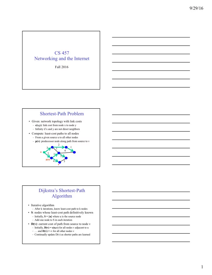
9/29/16 CS 457 Networking and the Internet Fall 2016 Shortest-Path Problem • Given: network topology with link costs – c(x,y) : link cost from node x to node y – Infinity if x and y are not direct neighbors • Compute: least-cost paths to all nodes – From a given source u to all other nodes – p(v) : predecessor node along path from source to v 2 1 3 1 4 u 2 1 5 p(v) 4 3 v Dijkstra’s Shortest-Path Algorithm • Iterative algorithm – After k iterations, know least-cost path to k nodes • S : nodes whose least-cost path definitively known – Initially, S = {u} where u is the source node – Add one node to S in each iteration • D(v) : current cost of path from source to node v – Initially, D(v) = c(u,v) for all nodes v adjacent to u – … and D(v) = ∞ for all other nodes v – Continually update D(v) as shorter paths are learned 1

9/29/16 Dijsktra’s Shortest Path Algorithm Notation: • c(x,y): link cost from node x to y; = 1 Initialization: ∞ if not direct neighbors 2 N' = {u} • D(v): current value of cost of path 3 for all nodes v from source to dest. v 4 if v adjacent to u • p(v): predecessor node along path from source to v 5 then D(v) = c(u,v) • N': set of nodes whose least cost 6 else D(v) = ∞ path is definitively known 7 8 Loop 9 find w not in N' such that D(w) is a minimum 10 add w to N' 11 update D(v) for all v adjacent to w and not in N' : 12 D(v) = min( D(v), D(w) + c(w,v) ) 13 /* new cost to v is either old cost to v or known 14 shortest path cost to w plus cost from w to v */ 15 until all nodes in N' Dijkstra’s Algorithm Example 2 2 1 1 3 3 1 1 4 4 2 2 1 1 5 5 4 4 3 3 2 2 1 1 3 3 1 1 4 4 2 2 1 1 5 5 4 4 3 3 Dijkstra’s Algorithm Example 2 2 1 1 3 3 1 1 4 4 2 2 1 1 5 5 4 4 3 3 2 2 1 1 3 3 1 1 4 4 2 2 1 1 5 5 4 4 3 3 2

9/29/16 Shortest-Path Tree • Shortest-path tree • Forwarding table from u at u 2 link v y 1 3 1 v (u,v) 4 x u z 2 w (u,w) 1 5 x (u,w) t 4 w 3 y (u,v) s z (u,v) s (u,w) t (u,w) Dijkstra’s Algorithm Limitations Algorithm complexity: n nodes • each iteration: need to check all nodes, w, not in N • n(n+1)/2 comparisons: O(n 2 ) • more efficient implementations possible: O(mlogn) Oscillations possible when link costs change: • e.g., link cost = amount of carried traffic A A A 1 A 1+e 2+e 0 0 2+e 2+e 0 D B 0 0 D B D B D B 1+e 1 0 0 1+e 1 0 e 0 0 1 1+e 0 e C C C C 1 1 e … recompute … recompute … recompute initially routing Link-State Routing • Each router keeps track of its incident links – Whether the link is up or down – The cost on the link • Each router broadcasts the link state – To give every router a complete view of the graph • Each router runs Dijkstra’s algorithm – To compute the shortest paths – … and construct the forwarding table • Example protocols – Open Shortest Path First (OSPF) – Intermediate System – Intermediate System (IS-IS) 3

9/29/16 Detecting Topology Changes • Beaconing – Periodic “hello” messages in both directions – Detect a failure after a few missed “hellos” “hello” • Performance trade-offs – Detection speed – Overhead on link bandwidth and CPU – Likelihood of false detection Broadcasting the Link State • Flooding – Node sends link-state information out its links – And then the next node sends out all of its links – … except the one where the information arrived X A X A C B D C B D (a) (b) X A X A C B D C B D (c) (d) Broadcasting the Link State • Reliable flooding – Ensure all nodes receive link-state information – … and that they use the latest version • Challenges – Packet loss – Out-of-order arrival • Solutions – Acknowledgments and retransmissions – Sequence numbers – Time-to-live for each packet 4

9/29/16 When to Initiate Flooding • Topology change – Link or node failure – Link or node recovery • Configuration change – Link cost change • Periodically – Refresh the link-state information – Typically (say) 30 minutes – Corrects for possible corruption of the data Convergence • Getting consistent routing information to all nodes – E.g., all nodes having the same link-state database • Consistent forwarding after convergence – All nodes have the same link-state database – All nodes forward packets on shortest paths – The next router on the path forwards to the next hop 2 1 3 1 4 2 1 5 4 3 Transient Disruptions • Detection delay – A node does not detect a failed link immediately – … and forwards data packets into a “blackhole” – Depends on timeout for detecting lost hellos 2 1 3 1 4 2 1 5 4 3 5

9/29/16 Transient Disruptions • Inconsistent link-state database – Some routers know about failure before others – The shortest paths are no longer consistent – Can cause transient forwarding loops 2 2 1 1 3 3 1 1 4 4 2 2 1 1 5 4 4 3 3 Convergence Delay • Sources of convergence delay – Detection latency – Flooding of link-state information – Shortest-path computation – Creating the forwarding table • Performance during convergence period – Lost packets due to blackholes and TTL expiry – Looping packets consuming resources – Out-of-order packets reaching the destination • Very bad for VoIP, online gaming, and video Reducing Convergence Delay • Faster detection – Smaller hello timers – Link-layer technologies that can detect failures • Faster flooding – Flooding immediately – Sending link-state packets with high-priority • Faster computation – Faster processors on the routers – Incremental Dijkstra algorithm • Faster forwarding-table update – Data structures supporting incremental updates 6

9/29/16 Comparison of LS and DV algorithms Message complexity Robustness: what happens if • LS: with n nodes, E links, router malfunctions? O(nE) messages sent LS: • DV: exchange between – Node can advertise neighbors only incorrect link cost – Each node computes only – Convergence time varies its own table Speed of Convergence DV: • LS: O(n 2 ) algorithm – DV node can advertise requires O(nE) messages incorrect path cost • DV: convergence time – Each node’s table used by others (error propagates) varies – May be routing loops – Count-to-infinity problem Summary • Routing is a distributed algorithm – React to changes in the topology – Compute the shortest paths • Two main shortest-path algorithms – Dijkstra à link-state routing (e.g., OSPF and IS-IS) – Bellman-Ford à distance vector routing (e.g., RIP) • Convergence process – Changing from one topology to another – Transient periods of inconsistency across routers Routing in Practice 7

9/29/16 RIP (Routing Information Protocol) • Distance vector algorithm • Included in BSD-UNIX Distribution in 1982 • Distance metric: # of hops (max = 15 hops) • Distance vectors: exchanged among neighbors every 30 sec via Response Message (also called advertisement ) • Each advertisement: list of up to 25 destination nets RIP: Example z w x y A D B C Destination Network Next Router Num. of hops to dest. w A 2 y B 2 z B 7 x -- 1 …. …. .... Routing table in D RIP: Example Dest Next hops Advertisement w - - from A to D x - - z C 4 …. … ... z w x y A D B C Destination Network Next Router Num. of hops to dest. w A 2 y B 2 z B A 7 5 x -- 1 …. …. .... Routing table in D 8

9/29/16 RIP: Link Failure and Recovery If no advertisement heard after 180 sec --> neighbor/link declared dead – routes via neighbor invalidated – new advertisements sent to neighbors – neighbors in turn send out new advertisements (if tables changed) – link failure info quickly propagates to entire net – poison reverse used to prevent ping-pong loops (infinite distance = 16 hops) RIP Table processing • RIP routing tables managed by application-level process called route-d (daemon) • advertisements sent in UDP packets, periodically repeated routed routed Transport Transport (UDP) (UDP) Network Network Forwarding Forwarding (IP) Table Table (IP) Link Link Physical Physical RIP Table example (continued) Router: giroflee.eurocom.fr Destination Gateway Flags Ref Use Interface -------------------- -------------------- ----- ----- ------ --------- 127.0.0.1 127.0.0.1 UH 0 26492 lo0 192.168.2. 192.168.2.5 U 2 13 fa0 193.55.114. 193.55.114.6 U 3 58503 le0 192.168.3. 192.168.3.5 U 2 25 qaa0 224.0.0.0 193.55.114.6 U 3 0 le0 default 193.55.114.129 UG 0 143454 ❒ Three attached networks (LANs) ❒ Router only knows routes to attached LANs ❒ Default router used to “go up” ❒ Route multicast address: 224.0.0.0 ❒ Loopback interface (for debugging) 9