
SLIDE 1
1
1
CS 331: Artificial Intelligence Fundamentals of Probability II
Thanks to Andrew Moore for some course material
2
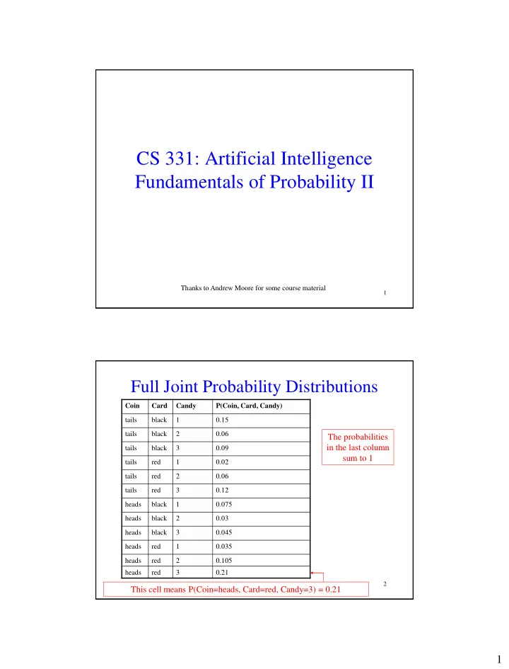
Full Joint Probability Distributions
Coin Card Candy P(Coin, Card, Candy) tails black 1 0.15 tails black 2 0.06 tails black 3 0.09 tails red 1 0.02 tails red 2 0.06 tails red 3 0.12 heads black 1 0.075 heads black 2 0.03 heads black 3 0.045 heads red 1 0.035 heads red 2 0.105 heads red 3 0.21
This cell means P(Coin=heads, Card=red, Candy=3) = 0.21 The probabilities in the last column sum to 1