craig m vineyard phd
play

Craig M. Vineyard, PhD Sandia National Laboratories is a - PowerPoint PPT Presentation

Photos placed in horizontal position with even amount of white space between photos and header Studying Adaptive Learning through Game-Theoretic Modeling Craig M. Vineyard, PhD Sandia National Laboratories is a multi-mission laboratory managed


  1. Photos placed in horizontal position with even amount of white space between photos and header Studying Adaptive Learning through Game-Theoretic Modeling Craig M. Vineyard, PhD 
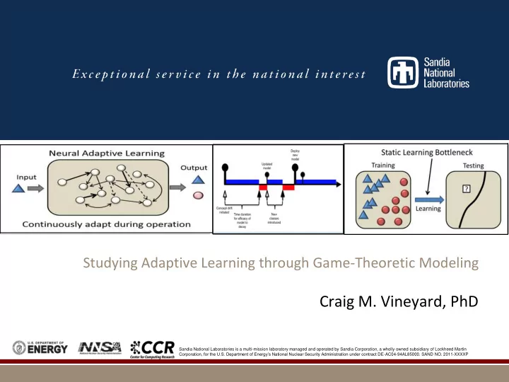
Sandia National Laboratories is a multi-mission laboratory managed and operated by Sandia Corporation, a wholly owned subsidiary of Lockheed Martin Corporation, for the U.S. Department of Energy’s National Nuclear Security Administration under contract DE -AC04-94AL85000. SAND NO. 2011-XXXXP

  2. Adaptive Learning  The learning phase of an algorithm addresses the mechanism by which adjustments are made in the learning process (such as weight tuning in a neural network)  One of the differentiating capabilities of the brain is continuous learning  So the question becomes where are we with respect to machine learning?  Most data-driven algorithms in ML do not continuously adapt 2

  3. ML Learning Paradigms …but they have limitations 3

  4. Static Learning Bottleneck 4

  5. Continuous Neural Adaptation  Synaptic plasticity  Dynamic alteration of the strength of the connections between neurons  Structural plasticity  Addition and eliminations of neural network infrastructure 5

  6. Game Theory  Game theory is a branch of applied mathematics to formally analyze the strategic interaction between competing players  Algorithmic Game Theory: the intersection of game theory & computer science • Analysis - analyzes algorithms from game-theoretic perspective, focus on properties such as equilibria • Design - focuses upon development of algorithms with desirable theoretical properties Why game theory?  Desirable properties for ML:  Leads to distributed computing, low overhead, simplicity, & provides a strategic perspective 6

  7. Moving Target Defense (MTD)  Use randomization, diversity, or change to make a computer system more difficult to attack (make it a “moving target”).  Randomized secret such as address-space layout randomization  Reset environment: new passwords, micro reboot, etc.  Deploy decoys. Change the real vs. decoys. KEY:  There is some information that helps the attacker as (s)he acquires it (e.g. in attempting to attack a system)  The defender can take this information away, at least temporarily 7

  8. PLADD  Probabilistic Learning Attacker Dynamic Defender (PLADD)  Extension of FlipIt attacker and defender model  Two players & one contested resource  A player can move at a cost  The “take” move - seizes control of the resource immediately  The “morph” move - resets the game  Neither player ever knows who owns the resource  Strategy: when to move? 8

  9. PLADD for Learning = FLANEL  Fundamental Learning Algorithm aNalysis and Exploration of Limits (FLANEL)  Modest extension that adds considerable complexity 9

  10. FLANEL  Morph = Rebuild the system (e.g. classifier)  Take = Short-term improvement PLADD with Varying probability distributions 10

  11. Exploring Alternatives to Simulation – vs – Analytical  Analysis continuum Simulation Stochastic Programming Analytical Increasing Flexibility, Expressiveness Increasing Generality  Challenges:  Analytical: optimal response over continuous (infinite) parameters  May require restrictive / unrealistic assumptions (e.g., periodic moves)  Simulation: enumerate (subset of) parameters and collect statistics  Search by full enumeration frequently computationally intractable  Opportunity:  Leverage numerical optimization to gain prescriptive insights while preserving much of the flexibility of simulation 11

  12. Method 1: Stochastic Programming  Key idea in stochastic programming:  approximate uncertainty by sampling outcomes  Approximate attacker’s strategy space by sampling possible random success-time outcomes  Attack scenarios  More scenarios gives a better approximation  Optimize to determine the defender’s single best strategy against ALL scenarios  Non-anticipative (only one solution for all attacks)  Extensive form is a mixed-integer program (MIP)  Can express more easily as a disjunctive program (DP)  Convert DP to MIP 12

  13. Stochastic Programming Example Idea:  Study the time between two major model rebuilds (morphs)  Fix the number of takes  Draw many concrete instantiations Distribution: Distribution: Time to lose trust Time to lose trust after full build after small fix 13

  14. Stochastic Program Example  Given many concrete scenarios (Explicit time to model failure) Given only k (3 in this case) small fixes, when to do them? • 14

  15. Stochastic Program Example  When to do the 3 small fixes? Never considered Cost from the PLADD model: average time when you cannot trust • the model. 15

  16. FLANEL Cost  When to do the 3 small fixes? = model untrusted Cost from the FLANEL model: average time when you cannot trust • the model. 16

  17. Method 2: Study Simpler Settings  Streaming setting Output Objects/data Classify, Answer arrive look up, etc.  Keep up with the stream  When the data structures in the box are badly tuned, too slow  Avoid dropping data elements 17

  18. Conclusion  Static Learning Bottleneck – need for adaptive learning  Working on a theoretical understanding of the problem  Need a holistic view not just Band-Aid solutions for individual problems  Mathematics of game theory are advantageous  Presented FLANEL as an adaptive learning analysis framework  Intended to provide a foundation for quantitatively evaluating adaptation in learning systems  Potential to impact how ML algorithms are implemented and deployed 18

  19. Thank you 19

  20. Backup Slides 20

  21. Interference  Google’s DeepMind announced in February 2015 that they’d built a system that could beat 49 Atari games  However, each time it beat a game the system needed to be retrained to beat the next one  "To get to artificial general intelligence we need something that can learn multiple tasks," says DeepMind researcher Hadsell . "But we can’t even Nature Vol 518 Number 7540 learn multiple games." 21

  22. Dynamic Environments  Concept Drift: changes in the data over time  Virtual: changes in the underlying data distribution  Real: concepts themselves are changing  Transfer Learning: the ability to utilize knowledge learned for one domain in learning a related but new domain 22

  23. Key Limitation “The development of game theory in the early 1940s by John von Neumann was a reaction against the then dominant view that problems in economic theory can be formulated using standard methods from optimization theory. Indeed, most real world economic problems typically involve conflicting interactions among decision-making agents that cannot be adequately captured by a single (global) objective function, thereby requiring a different, more sophisticated treatment .” M. Pelillo and A. Torsello  An analogous statement can be said about machine learning  Many learning problems involve dynamics that cannot be adequately capture by a single global objective function 23

  24. FlipIt Example  Two players: attacker and defender  One contested resource. Defender holds at start  A player can move at a cost  Takes resource (tie to defender)  Neither player ever knows who owns the resource  Strategy: when to move? Timeline is infinite.  Utility = (time in control) – cost (can be weighted) 24

  25. New Game: PLADD  Probabilistic Learning Attacker Dynamic Defender  Morphs reset to the start. Between morphs is a finite game  With no morphs, the game is infinite, like FlipIt  Difference between finite and infinite games is benefit of MTD finite 25

  26. Formulating and Solving Stochastic Programs … … … … ≡ … … … … … … … … … … … … t = 0 t = 1 t = 2 t = 0 t = 1 t = 2 Progressive Hedging Extensive Form optimize optimize = … … … … … … optimize optimize optimize optimize = … … … … … … = optimize … … … … … … optimize optimize = … … … … … … optimize t = 0 t = 1 t = 2 t = 0 t = 1 t = 2 26

  27. Extensive Formulation: MIP  One schedule/strategy to minimize average cost Compute costs for Scenario 1 Decision Compute costs Variables for Scenario 2 Compute costs for Scenario 3 Compute costs for Scenario 4 27

  28. Progressive Hedging Optimal individual decisions Lagrangian penalty terms 28

Download Presentation
Download Policy: The content available on the website is offered to you 'AS IS' for your personal information and use only. It cannot be commercialized, licensed, or distributed on other websites without prior consent from the author. To download a presentation, simply click this link. If you encounter any difficulties during the download process, it's possible that the publisher has removed the file from their server.

Recommend


More recommend