COST-MINIMIZATION C ( w, r, Q ) = min { w L + r K | F ( K, L ) Q } - - PDF document

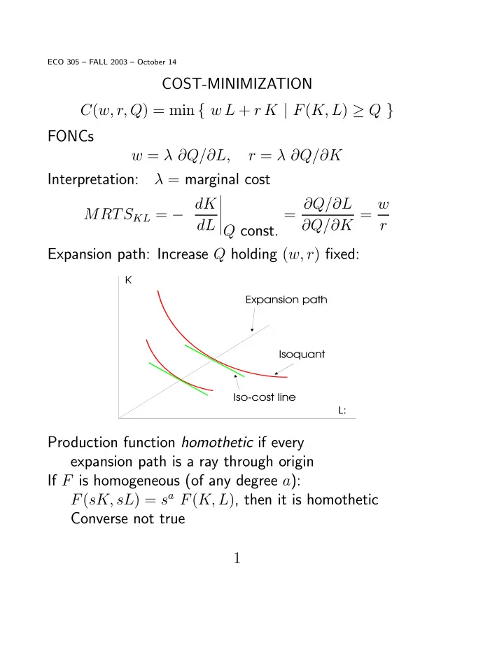
ECO 305 — FALL 2003 — October 14

COST-MINIMIZATION C(w, r, Q) = min { w L + r K | F(K, L) ≥ Q } FONCs w = λ ∂Q/∂L, r = λ ∂Q/∂K Interpretation: λ = marginal cost MRTSKL = − dK dL

¯ ¯ ¯ ¯ ¯Q const.

= ∂Q/∂L ∂Q/∂K = w r Expansion path: Increase Q holding (w, r) fixed: Production function homothetic if every expansion path is a ray through origin If F is homogeneous (of any degree a): F(sK, sL) = sa F(K, L), then it is homothetic Converse not true 1

PROPERTIES OF COST FUNCTION Vary Q holding (w, r) fixed — (ECO 102 material) Fixed cost: C(0) = 0, but as Q ↓ 0, lim C(Q) > 0 Sunk cost: C(0) > 0 AC(Q) = C(Q)/Q, MC(Q) = C0(Q) Returns to scale ↑ at margin: AC ↓, MC < AC returns to scale ↓ at margin: AC ↑; MC > AC If rets to scale first ↑, then ↓, U-shaped cost curves Vary (w, r) holding Q constant — (new material) Properties similar to consumer’s expenditure function (1) Homogeneous degree 1. (2) Concave, and (3) Hotelling’s (Shepherd’s) Lemma, cost-minimizing input choices are given by L∗ = ∂C/∂w, K∗ = ∂C/∂r 2

SHORT- AND LONG-RUN COST CURVES 3

4