A Minimization Algorithm Consider the minimization problem: * M - - PowerPoint PPT Presentation

A Minimization Algorithm

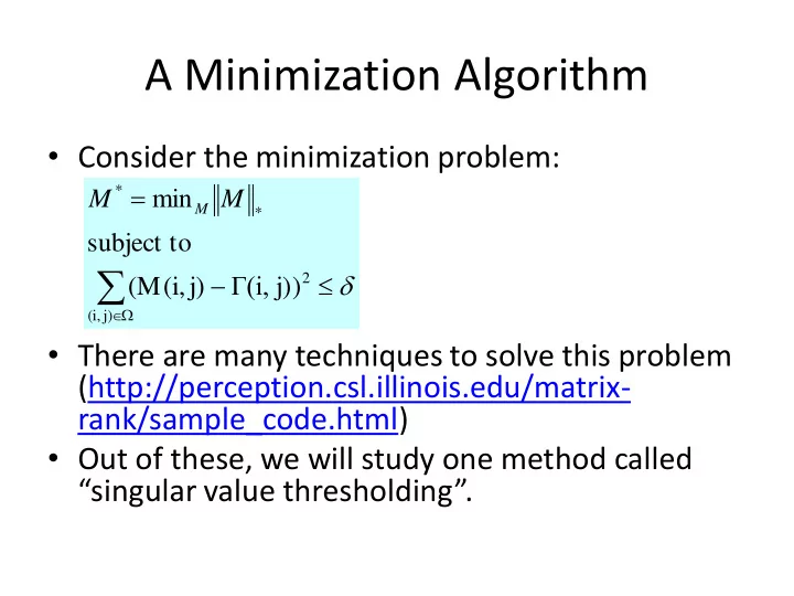
• Consider the minimization problem:
• There are many techniques to solve this problem

(http://perception.csl.illinois.edu/matrix- rank/sample_code.html)

• Out of these, we will study one method called

“singular value thresholding”.

   



  2 j) (i, * *

) j) Γ(i, j) (M(i, subject to min M M

M

Singular Value Thresholding (SVT)

Ref: Cai et al, A singular value thresholding algorithm for matrix completion, SIAM Journal

• n Optimization, 2010.

} ; } ; 1 ); ( ) ; ( { met) not criterion ergence while(conv 1 k { ) , (

) ( * ) ( ) 1 ( ) ( ) 1 ( ) ( ) ( *

2 1

k k k k k k k n n

k k P Y Y Y threshold soft R Y SVT                    

   

   } ) , ( ˆ } ); ) , ( , max( ) , ( { )) ( : 1 ( for ) svd using ( { ) ; ( ˆ

) ( 1

2 1



 

       

Y rank i t k k T n n

v u k k S Y k k S k k S Y rank k USV Y R Y threshold soft Y  

* 2

2 1 min arg ) ; ( X Y X Y threshold soft

F X

     

The soft- thresholding procedure obeys the following property (which we state w/o proof).

Properties of SVT (stated w/o proof)

• The sequence {k} converges to the true solution
• f the problem below provided the step-sizes {k}

all lie between 0 and 2.

• For large values of , this converges to the

solution of the original problem (i.e. without the Frobenius norm term).

) , ( ) , ( , ) , ( subject to 5 . min

2 * *

j i Γ j i M j i M M M

F M

      

Properties of SVT (stated w/o proof)

• The matrices {k} turn out to have low rank

(empirical observation – proof not established).

• The matrices {Yk} also turn out to be sparse

(empirical observation – rigorous proof not established).

• The SVT step does not require computation of

full SVD – we need only those singular vectors whose singular values exceed τ. There are special iterative methods for that.

Results

• The SVT algorithm works very efficiently and is

easily implementable in MATLAB.

• The authors report reconstruction of a 30,000

by 30,000 matrix in just 17 minutes on a 1.86 GHz dual-core desktop with 3 GB RAM and with MATLAB’s multithreading option enabled.

Results (Data without noise)

https://arxiv.org/abs/0810.3286

Results (Noisy Data)

https://arxiv.org/abs/0810.3286

Results on real data

• Dataset consists of a matrix M of geodesic

distances between 312 cities in the USA/Canada.

• This matrix is of approximately low-rank (in

fact, the relative Frobenius error between M and its rank-3 approximation is 0.1159).

• 70% of the entries of this matrix (chosen

uniformly at random) were blanked out.

Results on real data

https://arxiv.org/abs/0810.3286

Algorithm for Robust PCA

• The algorithm uses the augmented Lagrangian

technique.

• See

https://en.wikipedia.org/wiki/Augmented_Lag rangian_method and https://www.him.uni- bonn.de/fileadmin/him/Section6_HIM_v1.pdf

• Suppose you want to solve:

) ( , s.t. w.r.t. ) ( min    x c I i x x f

i

Algorithm for Robust PCA

• Suppose you want to solve:
• The augmented Lagrangian method (ALM)

adopts the following iterative updates:

) ( , s.t. w.r.t. ) ( min    x c I i x x f

i

) ( ) ( ) ( ) ( min arg

2 k i k i i I i i i I i i k x k

x c x c x c x f x          

 

 

Augmentation term Lagrangian term

ALM: Some intuition

• What is the intuition behind the update of the

Lagrange parameters {λi}?

• The problem is:

) ( I, i s.t. ) ( min    x c x f

i

)) ( ),..., ( ), ( ( ) ( ) ( ) ( max min

t

x c x c x c x x x f

| I | 2 1 x

  c c λ

λ

The maximum w.r.t. λ will be ∞ unless the constraint is satisfied. Hence these problems are equivalent.

ALM: Some intuition

• The problem is:

) ( I, i s.t. ) ( min    x c x f

i

)) ( ),..., ( ), ( ( ) ( ) ( ) ( max min

t

x c x c x c x x x f

| I | 2 1 x

  c c λ

λ

Due to non-smoothness of the max function, the equivalence has little computational benefit. We smooth it by adding another term that penalizes deviations from a prior estimate of the λ parameters.

 2 ) ( ) ( max min

2 t

λ

• λ

c λ

λ

  x x f

x

) (x c λ λ   

Maximization w.r.t. λ is now easy

ALM: Some inutuion – inequality constraints

) ( I, i s.t. ) ( min    x c x f

i

)) ( ),..., ( ), ( ( ) ( ) ( ) ( max min

t

x c x c x c x x x f

| I | 2 1 x

 



c c λ

λ

 2 ) ( ) ( max min

2 t

λ

• λ

c λ

λ

  x x f

x

) ), ( max( x c λ λ   

Maximization w.r.t. λ is now easy

Theorem 1 (Informal Statement)

• Consider a matrix M of size n1 by n2 which is the sum of a

“sufficiently low-rank” component L and a “sufficiently sparse” component S whose support is uniformly randomly distributed in the entries of M.

• Then the solution of the following optimization problem

(known as principal component pursuit) yields exact estimates of L and S with “very high” probability:



 

    

1 2

1 1 1 1 2 1 * ) , (

| | : . subject to ) , max( 1 min ) ' , ' (

n i n j ij S L

S S Note M S L S n n L S L E

This is a convex

• ptimization

problem.

Algorithm for Robust PCA

• In our case, we seek to optimize:
• Basic algorithm:

) ( ), , , ( min arg ) , (

1 ) , ( k k k k k S L k k

S L M Y Y Y S L l S L     





Lagrange matrix Update of S using soft-thresholding Update of L using singular-value soft-thresholding

Alternating Minimization Algorithm for Robust PCA

Results

https://statweb.stanford.edu/~candes/papers/RobustPCA.pdf

(Compressive) Low Rank Matrix Recovery

Compressive RPCA: Algorithm and an Application

Primarily based on the paper: Waters et al, “SpaRCS: Recovering Low-Rank and Sparse Matrices from Compressive Measurements”, NIPS 2011

Problem statement

• Let M be a matrix which is the sum of low rank

matrix L and sparse matrix S.

• We observed compressive measurements of

M in the following form:

y S L M y , S L S L y , given , Retrieve

• n

acting/map

• perator

linear , , ), (

2 1

2 1 2 1

A A A       

 

n n m R R R

m n n n n

Scenarios

• M could be a matrix representing a video –

each column of M is a vectorized frame from the video.

• M could also be a matrix representing a

hyperspectral image – each column is the vectorized form of a slice at a given wavelength.

• Robust Matrix completion – a special form of a

compressive L+S recovery problem.

Objective function: SpaRCS

Free parameters SpaRCS = sparse and low rank decomposition via compressive sampling

SparCS Algorithm

Very simple to implement; but requires tuning of K, r parameters; convergence guarantees not established. https://papers.nips.cc/pap er/4438-sparcs-recovering- low-rank-and-sparse- matrices-from- compressive- measurements.pdf

Results: Phase transition

https://papers.nips.cc/paper/4438-sparcs- recovering-low-rank-and-sparse-matrices- from-compressive-measurements.pdf Code: https://www.ece.rice.edu/~aew2/sparcs.html

Results: Video CS

Follows Rice SPC model, independent compressive measurements on each frame

• f the matrix M representing the video.

https://papers.nips.cc/paper/4438-sparcs- recovering-low-rank-and-sparse-matrices- from-compressive-measurements.pdf

Results: Video CS

Follows Rice SPC model, independent compressive measurements on each frame

• f the matrix M representing the video.

https://papers.nips.cc/paper/4438-sparcs- recovering-low-rank-and-sparse-matrices- from-compressive-measurements.pdf

Results: Hyperspectral CS

https://papers.nips.cc/paper/4438-sparcs-recovering-low-rank-and-sparse-matrices- from-compressive-measurements.pdf

Rice SPC model of CS measurements on every spectral band

Results: Robust matrix completion

https://papers.nips.cc/paper/4438-sparcs-recovering-low-rank-and-sparse- matrices-from-compressive-measurements.pdf

Theorem for Compressive PCP

Wright et al, “Compressive Principal Component Pursuit” http://yima.csl.illinois.edu/psfile/CPCP.pdf Q is obtained from the linear span

• f different independent N(0,1)

matrices with iid entries

Summary

• Low rank matrix completion: motivation, key

theorems, numerical results

• Algorithm for low rank matrix completion
• Robust PCA
• (Compressive) low rank matrix recovery
• Compressive RPCA
• Several papers linked on moodle