ARS Workshop Context Markov Random Fields minimization and minimal - - PowerPoint PPT Presentation

ARS Workshop Lucas Létocart Context Exact total variation minimization Total variation and regularization TV models Minimization Minimal cut (graph cut) as energy minimization Notations General principle Maximum flow / minimal cut Energy representation Results More results Further results for 3D images Conclusion Conclusion Perspectives 1

ARS Workshop

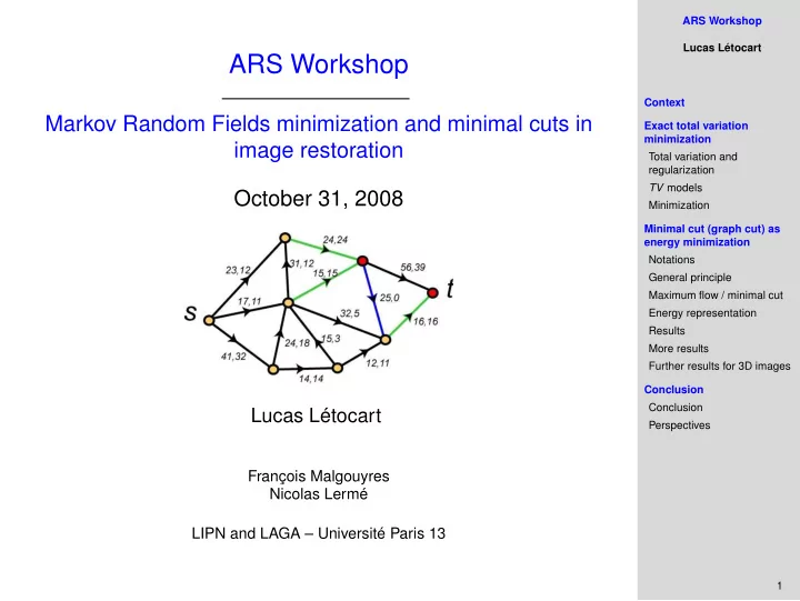
Markov Random Fields minimization and minimal cuts in image restoration October 31, 2008

Lucas Létocart

François Malgouyres Nicolas Lermé LIPN and LAGA – Université Paris 13

ARS Workshop Lucas Létocart Context Exact total variation minimization Total variation and regularization TV models Minimization Minimal cut (graph cut) as energy minimization Notations General principle Maximum flow / minimal cut Energy representation Results More results Further results for 3D images Conclusion Conclusion Perspectives 2

Outline

1

Context

2

Exact total variation minimization

Total variation and regularization TV models Minimization 3

Minimal cut (graph cut) as energy minimization

Notations General principle Maximum flow / minimal cut Energy representation Results More results Further results for 3D images 4

Conclusion

Conclusion Perspectives

ARS Workshop Lucas Létocart Context Exact total variation minimization Total variation and regularization TV models Minimization Minimal cut (graph cut) as energy minimization Notations General principle Maximum flow / minimal cut Energy representation Results More results Further results for 3D images Conclusion Conclusion Perspectives 3

Context

ARS Workshop Lucas Létocart Context Exact total variation minimization Total variation and regularization TV models Minimization Minimal cut (graph cut) as energy minimization Notations General principle Maximum flow / minimal cut Energy representation Results More results Further results for 3D images Conclusion Conclusion Perspectives 4

Main context

Image degradation v = Hu + η v → Observed image u → Original image η → Noise H → Linear degradation

Goal

Obtain the best estimation ¯ u from u when H = identity.

ARS Workshop Lucas Létocart Context Exact total variation minimization Total variation and regularization TV models Minimization Minimal cut (graph cut) as energy minimization Notations General principle Maximum flow / minimal cut Energy representation Results More results Further results for 3D images Conclusion Conclusion Perspectives 5

Energy minimization

First approach

Restoration corresponds to find the minimum of E(u, v) = X

p∈Ω

Fp(up, vp) with Ω ⊂ R2. Inverse problem (Hadamard) ⇒ noise amplification (when H = Id). Need to regularize the solution. E(u, v) = X

p∈Ω

Fp(up, vp) | {z }

Data fidelity term

+ β · X

p,q∈Ω {p,q}∈N

Gp,q(up, uq) | {z }

Regularization

∀β ∈ R+

∗

ARS Workshop Lucas Létocart Context Exact total variation minimization Total variation and regularization TV models Minimization Minimal cut (graph cut) as energy minimization Notations General principle Maximum flow / minimal cut Energy representation Results More results Further results for 3D images Conclusion Conclusion Perspectives 6

Energy minimization

Standard minimization methods

→ Continuous Gradient descent. Graduated Non Convexity (GCN). → Discrete Dynamic programming (only in 1D). Simulated annealing. Iterated Conditional Modes.

Problems

No or poor convergence guarantees. Solution not ever optimal.

ARS Workshop Lucas Létocart Context Exact total variation minimization Total variation and regularization TV models Minimization Minimal cut (graph cut) as energy minimization Notations General principle Maximum flow / minimal cut Energy representation Results More results Further results for 3D images Conclusion Conclusion Perspectives 7

Exact total variation minimization

ARS Workshop Lucas Létocart Context Exact total variation minimization Total variation and regularization TV models Minimization Minimal cut (graph cut) as energy minimization Notations General principle Maximum flow / minimal cut Energy representation Results More results Further results for 3D images Conclusion Conclusion Perspectives 8

Regularization

Regularization (Tikhonov)

From : Introduce by A. N. Tikhonov in 1963 Goal : Consider restoration as find the minimum of E(u) = u − v2

L2 + β · ∇u2 L2

where uLp = ( Z

Ω

|u(x)|p dx)

1 p

Problem

“Cubes” image σb = 30 Tikhonov restoration

Solution

Regularize differently. Decrease the weight of big gradients.

ARS Workshop Lucas Létocart Context Exact total variation minimization Total variation and regularization TV models Minimization Minimal cut (graph cut) as energy minimization Notations General principle Maximum flow / minimal cut Energy representation Results More results Further results for 3D images Conclusion Conclusion Perspectives 9

BV Space

Definition

BV ⇒ Space of functions with bounded variations. BV(Ω) = {u ∈ L1(Ω) | Z

Ω

|∇u| < +∞} Exact definition uses duality, because |∇u| can be a measure. with the semi-norm |u|BV = Z

Ω

|∇u| = TV(u) ⇒ Total Variation

Advantages

Discontinuities are authorized along curves. Good space for geometric images. Existence and unicity of the solution.

ARS Workshop Lucas Létocart Context Exact total variation minimization Total variation and regularization TV models Minimization Minimal cut (graph cut) as energy minimization Notations General principle Maximum flow / minimal cut Energy representation Results More results Further results for 3D images Conclusion Conclusion Perspectives 10

Total Variation

Definition (co-area – continuous )

Let u ∈ BV(Ω). Total variation of u is TV(u) = Z

Ω

|∇u| = Z

R

Z

d{u≤λ}

ds dλ, where {u ≤ λ} is equivalent to {u(x) ∈ Ω | u(x) ≤ λ}.

Definition (co-area – discrete)

Let u be a discrete function. Total variation of u is TV(u) =

L−2

X

λ=0

X

{p,q}∈N

wp,q|uλ

p − uλ q |

where uλ

p = 1{up≥λ}

Remarks

(-) Details suppression (textures). (+) Allows sharp contours.

ARS Workshop Lucas Létocart Context Exact total variation minimization Total variation and regularization TV models Minimization Minimal cut (graph cut) as energy minimization Notations General principle Maximum flow / minimal cut Energy representation Results More results Further results for 3D images Conclusion Conclusion Perspectives 11

TV models

Definition

Let v ∈ L1(Ω) the observed image. The TV model consist of finding argmin

u∈BV(Ω)

TV(u) + βu − vα

Lα

α ∈ {1, 2}

TV + L2 Model / ROF (Rudin Osher Fatemi 92)

(+) Strictly convex ⇒ unicity. (-) Lost of contrast (iterative regularization). Gaussian noise.

TV + L1 Model (Nikolova 2004)

(-) Convex ⇒ not unicity. (+) No contrast lost. Impulsive noise.

ARS Workshop Lucas Létocart Context Exact total variation minimization Total variation and regularization TV models Minimization Minimal cut (graph cut) as energy minimization Notations General principle Maximum flow / minimal cut Energy representation Results More results Further results for 3D images Conclusion Conclusion Perspectives 12

Level set approach

Principle

1 Decompose the image in order to solve a succession of quadratic binary

• ptimization problems ¯

uλ (MRF) 2 Solve each problem ¯ uλ where the solution is a level set 3 Reconstruct ¯ u from ¯ uλ (trivial)

Level set decomposition λ

Upper-set → Uλ(u) = {p ∈ Ω | up ≥ λ} Lower-set → Lλ(u) = {p ∈ Ω | up ≤ λ}

Reconstruction

up = sup{λ ∈ L | p ∈ Uλ(u)} ∀p ∈ Ω

ARS Workshop Lucas Létocart Context Exact total variation minimization Total variation and regularization TV models Minimization Minimal cut (graph cut) as energy minimization Notations General principle Maximum flow / minimal cut Energy representation Results More results Further results for 3D images Conclusion Conclusion Perspectives 13

Level set approach

Reformulation - TV + L1

argmin

uλ∈{0,1}N

Eλ

1 (uλ) = TV(uλ) + β

X

p∈Ω

[(1 − yp)uλ

p + yp(1 − uλ p )]

with yp = 1{vp≥λ}

Reformulation - TV + L2

argmin

uλ∈{0,1}N

Eλ

2 (uλ) = TV(uλ) + 2β

X

p∈Ω

“ (λ − 0.5)uλ

p + vp(1 − uλ p )

”

ARS Workshop Lucas Létocart Context Exact total variation minimization Total variation and regularization TV models Minimization Minimal cut (graph cut) as energy minimization Notations General principle Maximum flow / minimal cut Energy representation Results More results Further results for 3D images Conclusion Conclusion Perspectives 14

Level set approach

Reformulation

Here, MRF are positive-negative quadratic pseudo-boolean functions, ie all the linear terms are positive and all the quadratic terms are negative (equivalent to submodular functions). Solve MRF is thus equivalent to find a maximal independant set in a bipartite graph, ie find a maximal flow – minimal cut in an associated graph.

Theorem

Minimizing E is equivalent to minimizing all the Eλ for each level. Total energy E(u) = PL−2

λ=0 Eλ(uλ) can be minimized because { ¯

uλ}λ=0...L−2 is monotonous, ie: ¯ uλ ≤ ¯ uµ ∀λ < µ. The optimal solution is given by ∀p ∈ Ω, ¯ up = max{λ, ¯ uλ = 1}.

ARS Workshop Lucas Létocart Context Exact total variation minimization Total variation and regularization TV models Minimization Minimal cut (graph cut) as energy minimization Notations General principle Maximum flow / minimal cut Energy representation Results More results Further results for 3D images Conclusion Conclusion Perspectives 15

Minimal cut (graph cut) as energy minimization

ARS Workshop Lucas Létocart Context Exact total variation minimization Total variation and regularization TV models Minimization Minimal cut (graph cut) as energy minimization Notations General principle Maximum flow / minimal cut Energy representation Results More results Further results for 3D images Conclusion Conclusion Perspectives 16

Notations

G = (V, E) is a directed weighted graph with two terminals s, t where V = {1, . . . , k} ∪ {s} ∪ {t}, n = |V| E = {(i, j) | 1 ≤ i, j ≤ n, i = j}, m = |E| Capacity ⇒ c : E → R+ ∪ +∞ Flow ⇒ f : E → R

Vocabulary

Node s → source Node t → sink N-links → arcs (i, j) T-links → arcs (s, i) and (i, t) Example of a graph for a 3 × 3 image.

ARS Workshop Lucas Létocart Context Exact total variation minimization Total variation and regularization TV models Minimization Minimal cut (graph cut) as energy minimization Notations General principle Maximum flow / minimal cut Energy representation Results More results Further results for 3D images Conclusion Conclusion Perspectives 17

Definitions

Definition (flow)

Let G be a graph. f(i, j) must verify 1) Capacity constraints f(i, j) ≤ c(i, j) ∀i, j ∈ V et ∀(i, j) ∈ E 2) Flow symmetry f(i, j) = −f(j, i) ∀i, j ∈ V et ∀(i, j) ∈ E 3) Kirchhoff law P

j∈V−{s,t} (i,j)∈E

f(i, j) = 0 ∀i ∈ V − {s, t}

Definition (cut)

Cut is a partition C = (S, T ) of V such s ∈ S, t ∈ T et S ∩ T = ∅, S ∪ T = V

Definition (Cut capacity)

The capacity of a cut C is |C| = X

i∈S,j∈T (i,j)∈E

c(i, j)

ARS Workshop Lucas Létocart Context Exact total variation minimization Total variation and regularization TV models Minimization Minimal cut (graph cut) as energy minimization Notations General principle Maximum flow / minimal cut Energy representation Results More results Further results for 3D images Conclusion Conclusion Perspectives 18

General principle

Theorem (Energy minimization (Greig Porteous Seheult 89))

Let G = (V, E) be a directed weighted graph and E be an energy function.E can be minimized using a minimal cut in G for the image binary case.

Principle

1 Construct a graph G. 2 Compute a minimal cut C = (S, T ) in G ⇒ minimize E. 3 Assign a value to each up such that  up = 0 if p ∈ S up = 1 if p ∈ T

ARS Workshop Lucas Létocart Context Exact total variation minimization Total variation and regularization TV models Minimization Minimal cut (graph cut) as energy minimization Notations General principle Maximum flow / minimal cut Energy representation Results More results Further results for 3D images Conclusion Conclusion Perspectives 19

Maximum flow / minimal cut

Maximum flow algorithms

Augmenting paths Principle : Find iteratively a non saturated path from s to t in G. Algorithms : Ford-Fulkerson → O(m · f), where f = maximum flow Edmons-Karp → O(nm2) Dinic → O(n2m) Boykov-Kolmogorov → O(n2m|C|) Push-relabel Principe : Propagate an excess of flow repeatedly from s to t in G. Algorithms : General push flow relabel → O(n2m) Push flow relabel with dynamic trees → O(nmlog(n))

ARS Workshop Lucas Létocart Context Exact total variation minimization Total variation and regularization TV models Minimization Minimal cut (graph cut) as energy minimization Notations General principle Maximum flow / minimal cut Energy representation Results More results Further results for 3D images Conclusion Conclusion Perspectives 20

Energy representation

Questions

Which energies can be minimized via minimal cuts ? How construct the graph to minimize E ?

Definition (representation (Kolmogorov Zabih 02))

Let E be an energy function with n binary variables E(x1, . . . , xn) = X

i

Ei(xi) + X

i<j

Ei,j(xi, xj) with xi ∈ {0, 1}. Every function with one variable can be represented by a graph. Every function with two variables can be represented by a graph iff Ei,j(0, 0) + Ei,j(1, 1) ≤ Ei,j(0, 1) + Ei,j(1, 0) (submodular)

ARS Workshop Lucas Létocart Context Exact total variation minimization Total variation and regularization TV models Minimization Minimal cut (graph cut) as energy minimization Notations General principle Maximum flow / minimal cut Energy representation Results More results Further results for 3D images Conclusion Conclusion Perspectives 21

Energy representation

Energy Ei with Ei(0) < Ei(1) Energy Ei with Ei(0) > Ei(1) Energy Eij with C > A and C > D

ARS Workshop Lucas Létocart Context Exact total variation minimization Total variation and regularization TV models Minimization Minimal cut (graph cut) as energy minimization Notations General principle Maximum flow / minimal cut Energy representation Results More results Further results for 3D images Conclusion Conclusion Perspectives 22

Minimization algorithms

Sequential algorithm

Proposed by : Darbon, Chambolle, Zalesky. Principle : Do L independant optimizations. Complexity : O(L × F) with O(F) the complexity to find the maximal flow – minimal cut. Execution time : < 1 min.

Dyadic algorithm

Proposed by : Darbon, Chambolle, Hochbaum. Principle : Use the overlap between the level sets. Complexity : O(log2(L)).

ARS Workshop Lucas Létocart Context Exact total variation minimization Total variation and regularization TV models Minimization Minimal cut (graph cut) as energy minimization Notations General principle Maximum flow / minimal cut Energy representation Results More results Further results for 3D images Conclusion Conclusion Perspectives 23

Results

Tests caracteristics

Computer: AMD Athlon 64 X2 Dual Core 6000+, 2Go of RAM. Implementation under MegaWave2. Kolmogorov et al. library to compute the maximum flow. Images 2562 and 5122. Averages over 10 launchings.

Images

Image “Circles” Image “Man” Image “Elaine”

ARS Workshop Lucas Létocart Context Exact total variation minimization Total variation and regularization TV models Minimization Minimal cut (graph cut) as energy minimization Notations General principle Maximum flow / minimal cut Energy representation Results More results Further results for 3D images Conclusion Conclusion Perspectives 24

Results - TV + L1

Neighborhood: 4-connexity

Image Algorithm β = 0.25 β = 0.5 β = 1.0 β = 2.0 β = 4.0 “Circles” 2562 Sequential 0.07 0.07 0.06 0.06 0.06 Dyadic 0.11 0.09 0.09 0.09 0.08 “Circles” 5122 Sequential 0.29 0.27 0.27 0.27 0.27 Dyadic 0.41 0.37 0.36 0.36 0.36 “Man” 2562 Sequential 5.14 3.63 2.89 2.45 2.25 Dyadic 0.46 0.35 0.23 0.13 0.10 “Man” 5122 Sequential 19.65 14.18 11.73 10.30 9.67 Dyadic 1.89 1.37 0.92 0.54 0.43 “Elaine” 2562 Sequential 4.05 2.96 2.40 2.12 2.01 Dyadic 0.43 0.32 0.23 0.13 0.10 “Elaine” 5122 Sequential 15.85 11.67 9.97 9.14 8.71 Dyadic 1.98 1.37 0.95 0.56 0.43

Neighborhood: 8-connexity

Image Algorithm β = 0.25 β = 0.5 β = 1.0 β = 2.0 β = 4.0 “Circles” 2562 Sequential 0.23 0.18 0.16 0.16 0.16 Dyadic 0.37 0.26 0.23 0.22 0.21 “Circles” 5122 Sequential 0.79 0.67 0.64 0.64 0.63 Dyadic 1.19 0.94 0.87 0.85 0.85 “Man” 2562 Sequential 19.84 12.14 8.68 7.01 6.19 Dyadic 1.61 0.97 0.69 0.48 0.27 “Man” 5122 Sequential 74.19 44.80 35.66 27.97 25.01 Dyadic 6.94 3.93 2.89 1.85 1.10 “Elaine” 2562 Sequential 13.87 9.52 7.36 6.11 5.54 Dyadic 1.49 0.87 0.66 0.47 0.27 “Elaine” 5122 Sequential 56.59 36.39 27.48 24.17 22.57 Dyadic 6.15 3.75 2.63 1.89 1.12

ARS Workshop Lucas Létocart Context Exact total variation minimization Total variation and regularization TV models Minimization Minimal cut (graph cut) as energy minimization Notations General principle Maximum flow / minimal cut Energy representation Results More results Further results for 3D images Conclusion Conclusion Perspectives 25

Results - TV + L2

Neighborhood: 4-connexity

Image Algorithm β = 0.01 β = 0.02 β = 0.04 β = 0.08 β = 0.16 “Circles” 2562 Sequential 3.46 2.76 2.46 2.32 2.26 Dyadic 0.21 0.49 0.28 0.15 0.10 “Circles” 5122 Sequential 14.41 11.74 10.26 9.68 9.57 Dyadic 4.60 2.23 0.91 0.48 0.39 “Man” 2562 Sequential 4.03 3.36 2.96 2.70 2.55 Dyadic 0.55 0.39 0.30 0.24 0.20 “Man” 5122 Sequential 17.27 14.16 12.40 11.26 10.64 Dyadic 2.37 1.74 1.35 1.08 0.84 “Elaine” 2562 Sequential 4.01 3.34 2.91 2.64 2.47 Dyadic 0.53 0.42 0.33 0.26 0.20 “Elaine” 5122 Sequential 17.25 14.38 12.29 11.08 10.48 Dyadic 2.74 1.96 1.46 1.13 0.85

Neighborhood: 8-connexity

Image Algorithm β = 0.01 β = 0.02 β = 0.04 β = 0.08 β = 0.16 “Circles” 2562 Sequential 10.34 8.13 6.91 6.36 6.03 Dyadic 0.66 0.38 0.92 0.60 0.31 “Circles” 5122 Sequential 43.84 32.68 27.79 24.90 23.99 Dyadic 2.12 7.02 4.05 1.66 1.04 “Man” 2562 Sequential 11.24 9.24 7.98 7.23 6.75 Dyadic 1.00 0.90 0.73 0.57 0.48 “Man” 5122 Sequential 46.66 37.18 31.91 28.78 26.83 Dyadic 5.29 4.40 3.08 2.49 2.03 “Elaine” 2562 Sequential 11.06 9.25 8.02 7.30 6.77 Dyadic 1.09 0.89 0.77 0.62 0.51 “Elaine” 5122 Sequential 48.13 38.25 33.07 29.49 27.39 Dyadic 5.87 4.88 3.44 2.70 2.12

ARS Workshop Lucas Létocart Context Exact total variation minimization Total variation and regularization TV models Minimization Minimal cut (graph cut) as energy minimization Notations General principle Maximum flow / minimal cut Energy representation Results More results Further results for 3D images Conclusion Conclusion Perspectives 26

More results

Tests caracteristics

Impulsive noise: db = 20% and db = 40%. Gaussian noise: σb = 15 and σb = 30. Images 5122. Connexity 8.

Images

Image “Cubes” Image “Man”

ARS Workshop Lucas Létocart Context Exact total variation minimization Total variation and regularization TV models Minimization Minimal cut (graph cut) as energy minimization Notations General principle Maximum flow / minimal cut Energy representation Results More results Further results for 3D images Conclusion Conclusion Perspectives 27

Results - TV + L1 - db = 20%

Noise - SNR = 3.44 Result - β = 0.65 Level lines Bruit - SNR = 2.11 Result - β = 3.8

ARS Workshop Lucas Létocart Context Exact total variation minimization Total variation and regularization TV models Minimization Minimal cut (graph cut) as energy minimization Notations General principle Maximum flow / minimal cut Energy representation Results More results Further results for 3D images Conclusion Conclusion Perspectives 28

Results - TV + L1 - db = 40%

Noise - SNR = 0.47 Result - β = 0.65 Level lines Noise - SNR = −0.88 Result - β = 2.8

ARS Workshop Lucas Létocart Context Exact total variation minimization Total variation and regularization TV models Minimization Minimal cut (graph cut) as energy minimization Notations General principle Maximum flow / minimal cut Energy representation Results More results Further results for 3D images Conclusion Conclusion Perspectives 29

Results - TV + L2 - σb = 15

Noise - SNR = 14.70 Result - β = 0.04 Level lines Noise - SNR = 12.1 Result - β = 0.1

ARS Workshop Lucas Létocart Context Exact total variation minimization Total variation and regularization TV models Minimization Minimal cut (graph cut) as energy minimization Notations General principle Maximum flow / minimal cut Energy representation Results More results Further results for 3D images Conclusion Conclusion Perspectives 30

Results - TV + L2 - σb = 30

Noise - SNR = 8.82 Result - β = 0.03 Level lines Noise - SNR = 6.25 Result - β = 0.06

ARS Workshop Lucas Létocart Context Exact total variation minimization Total variation and regularization TV models Minimization Minimal cut (graph cut) as energy minimization Notations General principle Maximum flow / minimal cut Energy representation Results More results Further results for 3D images Conclusion Conclusion Perspectives 31

3D Images - Results - TV + L1

Image Algorithm β = 0.25 β = 0.5 β = 1.0 β = 2.0 β = 4.0 SPHERE-40 Sequential 0.10 0.05 0.04 0.04 0.04 Dyadic 0.60 0.17 0.18 0.15 0.15 SPHERE-40+db Sequential 17.98 11.56 6.92 5.95 6.12 Dyadic 0.72 0.22 0.20 0.20 0.21 SPHERE-80 Sequential 0.75 0.49 0.44 0.43 0.42 Dyadic 2.09 1.82 1.77 1.75 1.75 SPHERE-80+db Sequential 234.65 90.49 69.89 63.65 65.88 Dyadic 2.96 2.38 2.24 2.19 2.33 FACTORIES-40 Sequential 10.93 8.62 6.72 5.91 5.04 Dyadic 1.93 0.84 0.77 0.33 0.19 FACTORIES-40+db Sequential 10.41 9.21 7.31 6.43 5.59 Dyadic 0.95 0.96 0.79 0.37 0.19 FACTORIES-80 Sequential 154.71 96.00 73.69 62.15 55.72 Dyadic 19.42 12.38 5.60 3.18 1.96 FACTORIES-80+db Sequential 166.67 108.72 80.44 67.14 60.26 Dyadic 20.01 10.37 6.90 3.59 2.01

Table: Computation times (seconds) for TV + L1 with 6 connexity. 3D images: 403 and 803.

ARS Workshop Lucas Létocart Context Exact total variation minimization Total variation and regularization TV models Minimization Minimal cut (graph cut) as energy minimization Notations General principle Maximum flow / minimal cut Energy representation Results More results Further results for 3D images Conclusion Conclusion Perspectives 32

3D Images - Results - TV + L1

Image Algorithm β = 0.25 β = 0.5 β = 1.0 β = 2.0 β = 4.0 SPHERE-40 Sequential 0.51 0.49 0.46 0.22 0.16 Dyadic 3.53 3.40 3.14 0.68 0.62 SPHERE-40+db Sequential 110.38 110.06 106.39 56.08 28.82 Dyadic 4.73 4.48 3.78 0.97 0.84 SPHERE-80 Sequential 8.01 7.39 2.52 1.52 1.31 Dyadic 59.35 54.78 6.69 5.72 5.51 SPHERE-80+db Sequential 1802.33 1643.56 873.04 299.68 218.54 Dyadic 73.46 63.76 9.33 7.31 7.16 FACTORIES-40 Sequential 44.16 43.96 52.74 43.61 29.97 Dyadic 5.48 4.91 4.84 4.25 3.07 FACTORIES-40+db Sequential 42.76 42.42 46.45 45.33 32.96 Dyadic 5.48 5.12 7.77 5.48 3.72 FACTORIES-80 Sequential 587.27 1027.61 783.87 410.16 259.07 Dyadic 78.69 119.34 129.47 95.27 23.31 FACTORIES-80+db Sequential 530.08 720.27 819.68 477.99 286.81 Dyadic 73.00 168.33 141.93 65.86 29.39

Table: Computation times (seconds) for TV + L1 with 26

• connexity. 3D images: 403 and 803.

ARS Workshop Lucas Létocart Context Exact total variation minimization Total variation and regularization TV models Minimization Minimal cut (graph cut) as energy minimization Notations General principle Maximum flow / minimal cut Energy representation Results More results Further results for 3D images Conclusion Conclusion Perspectives 33

3D Images - Results - TV + L2

Image Algorithm β = 0.01 β = 0.02 β = 0.04 β = 0.08 β = 0.16 SPHERE-40 Sequential 7.52 6.19 5.55 5.34 5.05 Dyadic 0.15 0.15 0.15 0.15 0.15 SPHERE-40+db Sequential 7.29 6.18 5.74 5.46 5.36 Dyadic 0.45 0.40 0.35 0.38 0.32 SPHERE-80 Sequential 81.86 67.72 63.29 57.48 56.52 Dyadic 1.74 1.74 1.74 1.74 1.74 SPHERE-80+db Sequential 78.92 68.82 63.94 60.42 59.70 Dyadic 4.32 3.80 3.86 3.65 3.79 FACTORIES-40 Sequential 9.63 7.50 6.52 5.90 5.54 Dyadic 0.99 0.94 0.56 0.41 0.36 FACTORIES-40+db Sequential 9.60 7.64 6.69 6.04 5.62 Dyadic 0.99 0.88 0.55 0.40 0.35 FACTORIES-80 Sequential 110.99 83.62 71.53 64.97 60.73 Dyadic 19.58 11.02 6.34 5.14 4.50 FACTORIES-80+db Sequential 112.19 84.65 72.29 65.26 61.34 Dyadic 18.28 10.40 6.23 4.36 3.65 CELLULES-40 Sequential 6.33 6.72 6.00 5.46 5.19 Dyadic 0.93 1.18 0.89 0.55 0.54 CELLULES-80 Sequential 107.74 84.60 68.65 61.70 58.07 Dyadic 29.35 33.07 12.75 7.58 4.94

Table: Computation times (seconds) for TV + L2 with 6 connexity. 3D images: 403 and 803.

ARS Workshop Lucas Létocart Context Exact total variation minimization Total variation and regularization TV models Minimization Minimal cut (graph cut) as energy minimization Notations General principle Maximum flow / minimal cut Energy representation Results More results Further results for 3D images Conclusion Conclusion Perspectives 34

3D Images - Results - TV + L2

Image Algorithme β = 0.01 β = 0.02 β = 0.04 β = 0.08 β = 0.16 SPHERE-40 Sequential 66.48 42.82 30.55 24.54 21.71 Dyadic 0.65 0.61 0.60 0.61 0.60 SPHERE-40+db Sequential 64.45 41.20 29.81 25.01 22.64 Dyadic 2.32 2.19 1.85 1.66 1.56 SPHERE-80 Sequential 598.28 378.50 274.36 219.81 209.11 Dyadic 5.87 5.54 5.50 5.62 5.65 SPHERE-80+db Sequential 550.09 347.81 260.82 219.12 196.73 Dyadic 27.87 20.94 17.62 15.52 14.38 FACTORIES-40 Sequential 66.24 54.15 39.77 30.34 25.40 Dyadic 8.90 5.69 3.75 3.55 2.12 FACTORIES-40+db Sequential 65.75 54.01 39.59 30.29 25.75 Dyadic 8.59 5.68 3.86 3.22 2.15 FACTORIES-80 Sequential 1099.51 673.16 391.58 281.06 227.92 Dyadic 173.10 75.40 52.07 38.89 21.55 FACTORIES-80+db Sequential 1086.86 662.72 387.27 281.60 231.48 Dyadic 108.21 67.50 49.87 33.01 20.38 CELLULES-40 Sequential 23.09 23.98 24.71 26.91 24.28 Dyadic 3.05 3.43 3.76 5.24 3.03 CELLULES-80 Sequential 262.14 277.04 373.07 294.75 239.85 Dyadic 50.98 61.38 126.01 67.98 48.13

Table: Computation times (seconds) for TV + L2 with 26

• connexity. 3D images: 403 and 803.

ARS Workshop Lucas Létocart Context Exact total variation minimization Total variation and regularization TV models Minimization Minimal cut (graph cut) as energy minimization Notations General principle Maximum flow / minimal cut Energy representation Results More results Further results for 3D images Conclusion Conclusion Perspectives 35

Conclusion

ARS Workshop Lucas Létocart Context Exact total variation minimization Total variation and regularization TV models Minimization Minimal cut (graph cut) as energy minimization Notations General principle Maximum flow / minimal cut Energy representation Results More results Further results for 3D images Conclusion Conclusion Perspectives 36

Conclusion

TV minimization

(+) Exact solutions. (+) Quick results. (-) Restricted energy classes. (-) Over-smoothing along the discontinuities.

ARS Workshop Lucas Létocart Context Exact total variation minimization Total variation and regularization TV models Minimization Minimal cut (graph cut) as energy minimization Notations General principle Maximum flow / minimal cut Energy representation Results More results Further results for 3D images Conclusion Conclusion Perspectives 37

Perspectives

Parametric flow

Objectif : re-use the flow value. Conditions : Arcs (s, i) → non-increasing capacities. Arcs (i, t) → non-decreasing capacities. Arcs (i, j) → constant capacities. Results : Less improvements than for the dyadic technique (Darbon Chambolle 08). Applications : interactive segmentation, video segmentation.

ARS Workshop Lucas Létocart Context Exact total variation minimization Total variation and regularization TV models Minimization Minimal cut (graph cut) as energy minimization Notations General principle Maximum flow / minimal cut Energy representation Results More results Further results for 3D images Conclusion Conclusion Perspectives 38

Perspectives

Extension to multiway cut

Multi-labelling

Extension to other operators

Goal : generalize restoration to other operators H (convolution, sampling). Applications : confocal microscopy, IRM.

Extension to other energy minimization models

Potts model