convolution pyramids
play

Convolution Pyramids Zeev Farbman , Raanan Fattal and Dani Lischinski - PowerPoint PPT Presentation

Convolution Pyramids Zeev Farbman , Raanan Fattal and Dani Lischinski Motivation SIGGRAPH Asia Conference (2011) Convolution Pyramids Application 1 - Gaussian Kernels presented by: Julian Steil Application 2 - Boundary Interpolation


  1. Convolution Pyramids Zeev Farbman , Raanan Fattal and Dani Lischinski Motivation SIGGRAPH Asia Conference (2011) Convolution Pyramids Application 1 - Gaussian Kernels presented by: Julian Steil Application 2 - Boundary Interpolation supervisor: Application 3 - Gradient Integration Prof. Dr. Joachim Weickert Summary 
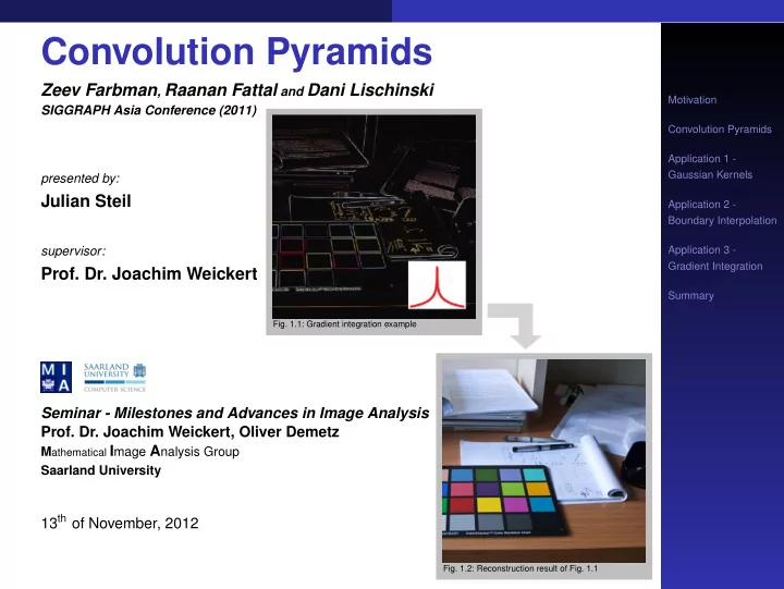
Fig. 1.1: Gradient integration example Seminar - Milestones and Advances in Image Analysis Prof. Dr. Joachim Weickert, Oliver Demetz M athematical I mage A nalysis Group Saarland University 13 th of November, 2012 Fig. 1.2: Reconstruction result of Fig. 1.1

  2. Overview Motivation 1. Motivation Convolution Pyramids 2. Convolution Pyramids Application 1 - Gaussian Kernels Application 2 - 3. Application 1 - Gaussian Kernels Boundary Interpolation Application 3 - 4. Application 2 - Boundary Interpolation Gradient Integration Summary 5. Application 3 - Gradient Integration 6. Summary

  3. Overview Motivation 1. Motivation Convolution Convolution Gaussian Pyramid Gaussian Pyramid Gaussian Pyramid - Example Gaussian Pyramid - Example From Gaussian to Laplacian From Gaussian to Laplacian Pyramid Pyramid Convolution Pyramids 2. Convolution Pyramids Application 1 - Gaussian Kernels 3. Application 1 - Gaussian Kernels Application 2 - Boundary Interpolation 4. Application 2 - Boundary Interpolation Application 3 - Gradient Integration 5. Application 3 - Gradient Integration Summary 6. Summary 2 / 22

  4. Motivation Convolution Motivation Two-Dimensional Convolution: Convolution • discrete convolution of two images Gaussian Pyramid Gaussian Pyramid - g = ( g i,j ) i,j ∈ Z and w = ( w i,j ) i,j ∈ Z : Example From Gaussian to Laplacian � � Pyramid ( g ∗ w ) i,j := g i − k,j − ℓ w k,ℓ (1) Convolution Pyramids k ∈ Z ℓ ∈ Z Application 1 - • components of convolution kernel w can be regarded as mirrored Gaussian Kernels weights for averaging the components of g Application 2 - Boundary Interpolation • the larger the kernel size the larger the runtime Application 3 - • ordinary convolution implementation needs O ( n 2 ) Gradient Integration Summary 3 / 22

  5. Motivation Gaussian Pyramid • sequence of images g 0 , g 1 , ..., g n Motivation • computed by a filtering procedure equivalent to convolution with a Convolution Gaussian Pyramid local, symmetric weighting function Gaussian Pyramid - = ⇒ e.g. a Gaussian kernel Example From Gaussian to Laplacian Procedure: Pyramid Convolution Pyramids • image initialised by array g 0 which contains C columns and R rows Application 1 - • each pixel represents the light intensity I between 0 and 255 Gaussian Kernels = ⇒ g 0 is the zero level of Gaussian Pyramid Application 2 - Boundary Interpolation • each pixel value in level i is computed as a weighting average of Application 3 - level i − 1 pixel values Gradient Integration Summary Fig. 2: One-dimensional graphic representation of the Gaussian pyramid 4 / 22

  6. Motivation Gaussian Pyramid - Example Motivation Convolution Gaussian Pyramid Gaussian Pyramid - Example From Gaussian to Laplacian Pyramid Convolution Pyramids Application 1 - Gaussian Kernels Application 2 - Boundary Interpolation Fig. 3: First six levels of the Gaussian pyramid for the “Lena” image. The original image, level 0, measures 257x257 pixels = ⇒ level 5 measures just 9x9 pixels Application 3 - Gradient Integration Summary Remark: density of pixels is reduced by half in one dimension and by fourth in two dimensions from level to level 5 / 22

  7. Motivation From Gaussian to Laplacian Pyramid Motivation Convolution Gaussian Pyramid Gaussian Pyramid - Example From Gaussian to Laplacian Pyramid Convolution Pyramids Application 1 - Gaussian Kernels Application 2 - Boundary Interpolation Application 3 - Gradient Integration Summary Fig. 4: First four levels of the Gaussian and Laplacian pyramid of Fig.3. • each level of Laplacian pyramid is the difference between the corresponding and the next higher level of the Gaussian pyramid • full expansion is used in Fig. 4 to help visualise the contents the pyramid images 6 / 22

  8. Overview Motivation 1. Motivation Convolution Pyramids Approach 2. Convolution Pyramids Forward and Backward Approach Transform Forward and Backward Transform Flow Chart and Pseudocode Flow Chart and Pseudocode Optimisation Optimisation Application 1 - Gaussian Kernels 3. Application 1 - Gaussian Kernels Application 2 - Boundary Interpolation 4. Application 2 - Boundary Interpolation Application 3 - Gradient Integration 5. Application 3 - Gradient Integration Summary 6. Summary 6 / 22

  9. Convolution Pyramids Approach Task: Motivation Convolution Pyramids • approximate effect of convolution with large kernels Approach = ⇒ higher spectral accuracy + translation-invariant operation Forward and Backward Transform • Is it also possible in O ( n )? Flow Chart and Pseudocode Optimisation Idea: Application 1 - • use of repeated convolution with small kernels on multiple scales Gaussian Kernels • disadvantage: not translation-invariant due to subsampling Application 2 - Boundary Interpolation operation to reach O ( n ) performance Application 3 - Gradient Integration Method: Summary • pyramids rely on a spectral “divide-and-conquer” strategy • no subsampling of the decomposed signal increases the translation-invariance • use finite impulse response filters to achieve some spacial localisation and runtime O ( n ) 7 / 22

  10. Convolution Pyramids Approach Task: Motivation Convolution Pyramids • approximate effect of convolution with large kernels Approach = ⇒ higher spectral accuracy + translation-invariant operation Forward and Backward Transform • Is it also possible in O ( n )? Flow Chart and Pseudocode Optimisation Idea: Application 1 - • use of repeated convolution with small kernels on multiple scales Gaussian Kernels • disadvantage: not translation-invariant due to subsampling Application 2 - Boundary Interpolation operation to reach O ( n ) performance Application 3 - Gradient Integration Method: Summary • pyramids rely on a spectral “divide-and-conquer” strategy • no subsampling of the decomposed signal increases the translation-invariance • use finite impulse response filters to achieve some spacial localisation and runtime O ( n ) 7 / 22

  11. Convolution Pyramids Approach Task: Motivation Convolution Pyramids • approximate effect of convolution with large kernels Approach = ⇒ higher spectral accuracy + translation-invariant operation Forward and Backward Transform • Is it also possible in O ( n )? Flow Chart and Pseudocode Optimisation Idea: Application 1 - • use of repeated convolution with small kernels on multiple scales Gaussian Kernels • disadvantage: not translation-invariant due to subsampling Application 2 - Boundary Interpolation operation to reach O ( n ) performance Application 3 - Gradient Integration Method: Summary • pyramids rely on a spectral “divide-and-conquer” strategy • no subsampling of the decomposed signal increases the translation-invariance • use finite impulse response filters to achieve some spacial localisation and runtime O ( n ) 7 / 22

  12. Convolution Pyramids Forward and Backward Transform Forward Transform - Analysis Step: Motivation • convolve a signal with a first filter h 1 Convolution Pyramids Approach • subsample the result by a factor of two Forward and Backward Transform • process is repeated on the subsampled data Flow Chart and • an unfiltered and unsampled copy of the signal is kept at each level Pseudocode Optimisation a l 0 = a l (2) Application 1 - Gaussian Kernels a l +1 = ↓ ( h 1 ∗ a l ) (3) Application 2 - Boundary Interpolation Application 3 - Backward Transform - Synthesis Step: Gradient Integration • upsample by inserting a zero between every two samples Summary • convolve the result with a second filter h 2 • combine upsampled signal with the signal stored at each level after convolving with a third filter g a l = h 2 ∗ ( ↑ ˆ a l +1 ) + g ∗ a l ˆ (4) 0 8 / 22

  13. Convolution Pyramids Forward and Backward Transform Forward Transform - Analysis Step: Motivation • convolve a signal with a first filter h 1 Convolution Pyramids Approach • subsample the result by a factor of two Forward and Backward Transform • process is repeated on the subsampled data Flow Chart and • an unfiltered and unsampled copy of the signal is kept at each level Pseudocode Optimisation a l 0 = a l (2) Application 1 - Gaussian Kernels a l +1 = ↓ ( h 1 ∗ a l ) (3) Application 2 - Boundary Interpolation Application 3 - Backward Transform - Synthesis Step: Gradient Integration • upsample by inserting a zero between every two samples Summary • convolve the result with a second filter h 2 • combine upsampled signal with the signal stored at each level after convolving with a third filter g a l = h 2 ∗ ( ↑ ˆ a l +1 ) + g ∗ a l ˆ (4) 0 8 / 22

Download Presentation
Download Policy: The content available on the website is offered to you 'AS IS' for your personal information and use only. It cannot be commercialized, licensed, or distributed on other websites without prior consent from the author. To download a presentation, simply click this link. If you encounter any difficulties during the download process, it's possible that the publisher has removed the file from their server.

Recommend


More recommend