Convolution matrix reversed impulse response impulse response - PDF document

1 Mathematical Tools for Neural and Cognitive Science Fall semester, 2018 Section 3: Linear Shift-invariant Systems 2 Linear shift-invariant (LSI) systems • Linearity (previously discussed): “linear combination in, linear combination out” • Shift-invariance (new property): “shifted vector in, shifted vector out” • Note: These two properties are independent (think of some examples that have both, one, or neither) 3 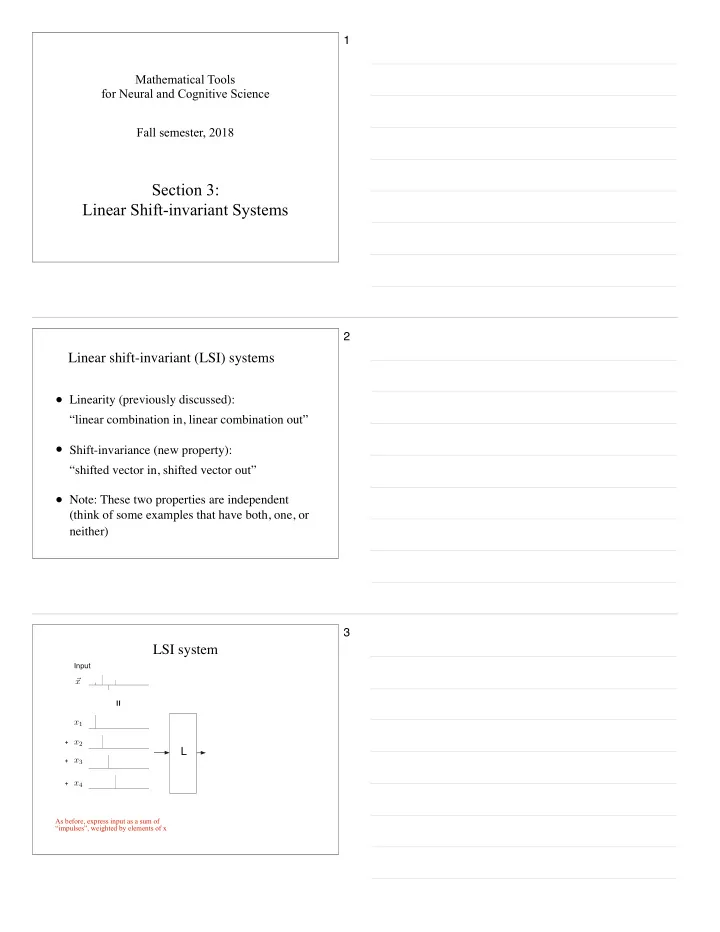LSI system Input v v1 x v1 x v2 x v2 x + + L + v3 x + v3 x v4 x + + v4 x Output As before, express input as a sum of “impulses”, weighted by elements of x

4 LSI system Input v v1 x v1 x v2 x v2 x + + L v3 x + + v3 x + v4 x + v4 x • Linearity => response to x is sum of Output responses to impulses, weighted by elements of x • Shift-invariance => responses to impulses are shifted copies of each other 5 LSI system Input v v1 x v1 x v2 x v2 x + + L v3 x + + v3 x v4 x + + v4 x Output LSI systems are characterized by their “impulse response” 6 Convolution In r 2 r 3 r 2 r 1 r r 0 1 X y ( n ) = r ( n − k ) x ( k ) + + k X = r ( k ) x ( n − k ) Out k • Sliding dot product • Structured matrix • Boundaries? zero-padding, reflection, circular • Examples: impulse, delay, average, difference

7 Convolution matrix reversed impulse response impulse response boundaries? 8 Feedback LSI system In • Response depends on input, and r 3 r 2 r 1 previous outputs + • Infinite impulse response (IIR) • Recursive => possibly unstable Out X X y ( n ) = f ( n − k ) x ( k ) + g ( n − k ) y ( k ) k k (For this class, we’ll stick to feedforward (FIR) systems) 9 2D convolution “sliding window” [figure c/o Castleman]

10 Discrete Sinusoids “frequency” (cycles/vectorLength) 1 cos( ω n ) , ω = 2 π k/N 0 − 1 0 10 20 30 “frequency” (radians/sample) example : A = 1 . 5 , φ = 8 π / 32 2 1 More generally: 0 − 1 “amplitude” − 2 0 10 20 30 “phase” (radians) 11 Shifting Sinusoids A cos( ω n − φ ) = A cos( φ ) cos( ω n ) + A sin( φ ) sin( ω n ) ... via a well-known trigonometric identity: cos( a − b ) = cos( a ) cos( b ) + sin( a ) sin( b ) We’ll also need conversions between polar and rectangular coordinates: y x = A cos( φ ) , y = A sin( φ ) A φ x 2 + y 2 , p φ = tan − 1 ( y/x ) A = x 12 Shifting Sinusoids A cos( ω n − φ ) = A cos( φ ) cos( ω n ) + A sin( φ ) sin( ω n ) fixed cos/sin vectors: scale factors: 1 0 A sin φ A − 1 0 10 20 30 1 φ A cos φ 0 − 1 0 10 20 30 Any scaled and shifted sinusoidal vector can be written as a weighted sum of two fixed {sin, cos} vectors!

13 Shifting Sinusoids A cos( ω n − φ ) = A cos( φ ) cos( ω n ) + A sin( φ ) sin( ω n ) fixed cos/sin vectors: A = 1.6, φ = 2 π 0/12 A = 1.6, φ = 2 π 1/12 1 0 1 1 − 1 0 10 20 30 0 0 1 − 1 − 1 − 1 0 0 0 0 10 10 10 20 20 20 30 30 30 − 1 0 10 20 30 Any scaled and shifted sinusoidal vector can be written as a weighted sum of two fixed {sin, cos} vectors! 14 Shifting Sinusoids A cos( ω n − φ ) = A cos( φ ) cos( ω n ) + A sin( φ ) sin( ω n ) fixed cos/sin vectors: A = 1.6, φ = 2 π 4/12 A = 1.6, φ = 2 π 2/12 A = 1.6, φ = 2 π 3/12 A = 1.6, φ = 2 π 5/12 A = 1.6, φ = 2 π 6/12 1 0 1 1 1 1 1 − 1 0 10 20 30 0 0 0 0 0 1 − 1 − 1 − 1 − 1 − 1 − 1 0 0 0 0 0 0 10 10 10 10 10 20 20 20 20 20 30 30 30 30 30 0 10 20 30 − 1 0 10 20 30 Any scaled and shifted sinusoidal vector can be written as a weighted sum of two fixed {sin, cos} vectors! 15 LSI response to sinusoids x ( n ) = cos( ω n ) (input)

16 LSI response to sinusoids x ( n ) = cos( ω n ) (convolution formula) L 17 LSI response to sinusoids x ( n ) = cos( ω n ) (trig identity) inner product of impulse response with cos/sin, respectively L 18 LSI response to sinusoids x ( n ) = cos( ω n ) L

19 LSI response to sinusoids x ( n ) = cos( ω n ) (rectangular -> polar coordinates) A sin φ s r ( ω ) R s ( ω ) A φ A cos φ c r ( ω ) R c ( ω ) 20 LSI response to sinusoids x ( n ) = cos( ω n ) (trig identity, in the opposite direction) L “Sinusoid in, sinusoid out” (with modified amplitude & phase) 21 LSI response to sinusoids More generally, if input has amplitude and phase , A x φ x then linearity and shift-invariance tell us that amplitudes multiply phases add L “Sinusoid in, sinusoid out” (with modified amplitude & phase)

22 The Discrete Fourier transform (DFT) • Construct an orthogonal matrix of sin/cos pairs, covering different numbers of cycles • Frequency multiples of radians/sample, 
 (specifically, ) • For , only need the cosine part (thus, cosines, and sines) N/ 2 + 1 N/ 2 − 1 • When we apply this matrix to an input vector, think of output as paired coordinates • Common to plot these pairs as amplitude/phase [details on board...] 23 Fourier Transform matrix k =0 k =1 k =2 k =3 k =N/2 F = cos ( sin ( 2 π k N n ) 2 π k N n ) (plotted sinusoids are continuous, N=32) 24 The Fourier family signal domain frequency domain (we are here) The “fast Fourier transform” (FFT) is a computationally efficient implementation of the DFT, requiring Nlog(N) operations, compared to the N 2 operations that would be needed for matrix multiplication.

25 LSI response to sinusoids x ( n ) = cos( ω n ) NOTE: These dot products are the Fourier transform of the impulse response, r(m) ! 26 Fourier & LSI ⇥ L x 27 Fourier & LSI ⇥ L x note: only 3 (of many) frequency components shown

28 Fourier & LSI ⇥ L x note: only 3 (of many) frequency components shown 29 Fourier & LSI Input ⇥ L x v v1 x v1 x v2 x + + v2 x L + v3 x + v3 x v4 x + + v4 x Output LSI systems are characterized by their frequency response , specified by the Fourier Transform of their impulse response 30 Complex exponentials: “bundling” sine and cosine e i θ = cos( θ ) + i sin( θ ) e i ω n = cos( ω n ) + i sin( ω n ) real part: n imaginary part: n [on board: reminders of addition/multiplication of complex numbers]

31 Complex exponentials: “bundling” sine and cosine e i ω n L F.T. of impulse response! 32 Complex exponentials: “bundling” sine and cosine e i ω n L F.T. of impulse response! L Note: the complex exponentials are eigenvectors ! 33 The “convolution theorem” convolve with

34 The “convolution theorem” convolve with Fourier Transform Fourier Transform inverse pointwise multiply by 35 The “convolution theorem” L convolve with Fourier Transform Fourier Transform inverse F T F pointwise multiply by F T ~ y = ˜ RF T ~ x ⇒ (diagonal matrix) 36 Recap… • Linear system - defined by superposition - characterized by a matrix • Linear Shift-Invariant (LSI) system - defined by superposition and shift-invariance - characterized by a vector (the impulse response) - OR, characterized by frequency response. Specifically, the Fourier Transform of the impulse response specifies an amplitude multiplier and a phase shift for each frequency.

37 Discrete Fourier transform (with complex numbers) ω k = 2 π k where N N − 1 r n = 1 X r k e i ω k n ˜ (inverse) N k =0 k Redraw with spiral included! [on board: why minus sign? why 1/N?] 38 Visualizing the (Discrete) Fourier Transform • Two conventional choices for frequency axis: - Plot frequencies from k=0 to k=N/2 (in matlab: 1 to N/2-1) - Plot frequencies from k=-N/2 to N/2-1 (in matlab: use fftshift) • Typically, plot amplitude (and possibly phase , on a separate graph), instead of the real/ imaginary (cosine/sine) components 39 More examples • constant • sinusoid (see next slide) • impulse • Gaussian - “lowpass” • DoG (difference of 2 Gaussians) - “bandpass” • Gabor (Gaussian windowed sinusoid) - “bandpass” [on board]

40 => Example for k=2, N=32 (note indexing and amplitudes): 1 10 10 0 0 0 (real part) − 10 − 10 − 1 0 10 20 30 0 10 20 30 − 10 0 10 k 1 10 10 0 0 0 (imag part) − 10 − 10 − 1 0 10 20 30 0 10 20 30 − 10 0 10 k 41 What do we do with Fourier Transforms? • Represent/analyze periodic signals • Analyze/design LSI systems . In particular, how do you identify the nullspace? 42 Retinal ganglion cells (1D) Enroth-Cugell and Robson (1984)

43 Sampling causes “aliasing” Sampling process is linear, but many-to-one (non-invertible) “Aliasing” - one frequency masquerades as another [on board] Given the samples, it is common/natural to assume, or enforce, that they arose from the lowest compatible frequency... 44 Effect of sampling on the Fourier Transform: Sum of shifted copies | X ( ω ) | | X s ( ω ) | 45 Real-world aliasing downsample by 2 “Moiré pattern”

46 Pre-filtering to avoid spectral overlap (“aliasing”) L ( ω ) | X ( ω ) | lowpass filter, L ( ω ) cutoff at π / ∆ | X s ( ω ) | 47 Real-world aliasing downsample by 2 , with pre-filtering