CONSUMER PREFERENCES AND UTILITY De fi ned over conumption set of - PDF document

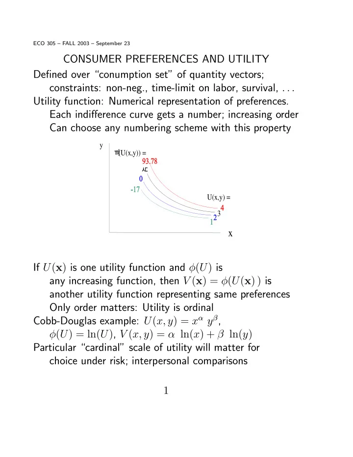
ECO 305 — FALL 2003 — September 23 CONSUMER PREFERENCES AND UTILITY De fi ned over “conumption set” of quantity vectors; constraints: non-neg., time-limit on labor, survival, . . . Utility function: Numerical representation of preferences. Each indi ff erence curve gets a number; increasing order Can choose any numbering scheme with this property y N (U(x,y)) = B U(x,y) = 3 x If U ( x ) is one utility function and φ ( U ) is any increasing function, then V ( x ) = φ ( U ( x ) ) is another utility function representing same preferences Only order matters: Utility is ordinal Cobb-Douglas example: U ( x, y ) = x α y β , φ ( U ) = ln( U ) , V ( x, y ) = α ln( x ) + β ln( y ) Particular “cardinal” scale of utility will matter for choice under risk; interpersonal comparisons 1

FORMAL STATEMENT: Notation: Preferred x  y , Indi ff erent x ∼ y Requirements of rationality: (1) Complete: for any x , y , x  y or y  x or x ∼ y (2) Re fl exive: for any x , x ∼ x (3) Transitive: If x  y and y  z , then x  z (4) Continuous: If x  y and z “near” y , then x  z Theorem: These there imply that there is a function U such that U ( x ) > U ( y ) if and only if x  y . MARGINAL RATE OF SUBSTITUTION Solve u = U ( x, y ) to get y = f ( x, u ) . (Numerical) slope ¯ ¯ MRS yx = − dy = ∂ U/ ∂ x ¯ ¯ ¯ dx ∂ U/ ∂ y U = constant MRS independent of cardinal utility: If V ( x, y ) = φ ( U ( x, y ) ) , ∂ V/ ∂ y = φ 0 ( U ) ∂ U/ ∂ x ∂ V/ ∂ x φ 0 ( U ) ∂ U/ ∂ y = ∂ U/ ∂ x ∂ U/ ∂ y Diminishing MRS: As x ↑ and y ↓ holding U constant, MRS decreases (indi ff erence curve becomes fl atter). SOSC for utility max subject to linear budget constraint Equivalent statement — If x ∼ y , then 1 2 ( x + y )  x , y 2

UTILITY MAXIMIZATION To maximize U ( x, y ) subject to P x x + P y y ≤ M . Budget constraint will be binding if “non-satiation” Lagrange FONCs for interior maximum L ( x, y ) = U ( x, y ) + λ [ M − P x x − P y y ] ∂ L/ ∂ x = ∂ U/ ∂ x − λ P x = 0 ∂ L/ ∂ y = ∂ U/ ∂ y − λ P y = 0 INTERPRETATIONS If ( x ∗ , y ∗ ) are optimum qunatities and u ∗ = U ( x ∗ , y ∗ ) , then λ = du ∗ /dM , “marginal utility of money” An extra dollar of income will buy you either 1 /P x of x or 1 /P y of y Respective utility increments from these are ∂ U/ ∂ x ∂ U/ ∂ y and P x P y Equal because of optimization; common value is the extra utility yielded by the extra dollar λ P x is “marginal (utility) cost” of buying x FONC: marginal (utility) bene fi t - marginal cost = 0 3

FONC for boundary optimum (0 , y ∗ ) ∂ L/ ∂ x = ∂ U/ ∂ x − λ P x ≤ 0 ∂ L/ ∂ y = ∂ U/ ∂ y − λ P y = 0 ∂ U/ ∂ x ≤ ∂ U/ ∂ y = λ P x P y Last dollar spent on y yields utility ( ∂ U/ ∂ y ) /P y = λ First dollar spent on x would yield ( ∂ U/ ∂ x ) /P x , less (GENERALIZED) DEMAND FUNCTIONS Optimum quantity choices x = D x ( P x , P y , M ) , y = D y ( P x , P y , M ) Marshallian or uncompensated or gross demand functions Simplest properties: (1) Adding up: P x D x ( P x , P y , M )+ P y D y ( P x , P y , M ) ≡ M (2) Homogeneity of degree zero: D x ( k P x , k P y , k M ) = D x ( P x , P y , M ) Budget constraint una ff ected; no money illusion (3) Don’t depend on cardinal utility: If V ( x, y ) = φ ( U ( x, y ) ) , and µ is Lagrange multiplier when maxing V ( x, y ) , ∂ V/ ∂ x = µ P x , ∂ V/ ∂ y = µ P y φ 0 ( U ) ∂ U/ ∂ x = µ P x , φ 0 ( U ) ∂ U/ ∂ y = µ P y same as FONCs for maxing U ( x, y ) with µ/ φ 0 ( U ) = λ 4

COBB-DOUGLAS EXAMPLE To max U ( x, y ) = x α y β , FONCs are ∂ U/ ∂ x ≡ α x α − 1 y β = λ P x , ∂ U/ ∂ y ≡ β x α y β − 1 = λ P y = x α y β P x x = P y y α β λ M = P x x + P y y = ( α + β ) x α y β λ P x x = P y y M = α β α + β P x x α P y y β = α + β , = M M α + β Proportions or shares of income spent on the two goods are constants. Check: (1) No boundary optima: U (0 , y ) = U ( x, 0) = 0 whereas U ( x, y ) > 0 when both x , y are positive. (2) Second Order Conditions: Indi ff erence curves convex: x α y β = u, y = u 1 / β x − α / β Exercise: Use V ( x, y ) = α ln( x ) + β ln( y ) and fi nd (1) same demand functions; (2) relation between multipliers 5

Income-Consumption Curve: Price-Consumption Curve: y y x x Algebraic concepts: ∆ M / M → M ∆ x / x ∂ x Income elasticity: x ∂ M ∆ x / x → P x ∂ x Own Price elasticity: ∆ P x / P x x ∂ P x ∆ x / x → P y ∂ x Cross-Price elasticity: ∆ P y / P y x ∂ P y Income elasticity < 0 : inferior, > 0 : normal, > 1 : luxury between 0 and 1: necessity Own Price elasticity > 0 : Gi ff en Cross-price elasticity > 0 : Marshallian or gross substitues < 0 : Marshallian or gross complements General concept : Comparative statics 6