Rational preferences Idea: preferences of a rational agent must obey - PDF document

Rational preferences Idea: preferences of a rational agent must obey constraints. Rational preferences ⇒ behavior describable as maximization of expected utility Rational decisions Constraints: Orderability ( A ≻ B ) ∨ ( B ≻ A ) ∨ ( A ∼ B ) Transitivity Chapter 16 ( A ≻ B ) ∧ ( B ≻ C ) ⇒ ( A ≻ C ) Continuity A ≻ B ≻ C ⇒ ∃ p [ p, A ; 1 − p, C ] ∼ B Substitutability A ∼ B ⇒ [ p, A ; 1 − p, C ] ∼ [ p, B ; 1 − p, C ] Monotonicity A ≻ B ⇒ ( p ≥ q ⇔ [ p, A ; 1 − p, B ] ≻ ∼ [ q, A ; 1 − q, B ]) Chapter 16 1 Chapter 16 4 Outline Rational preferences contd. 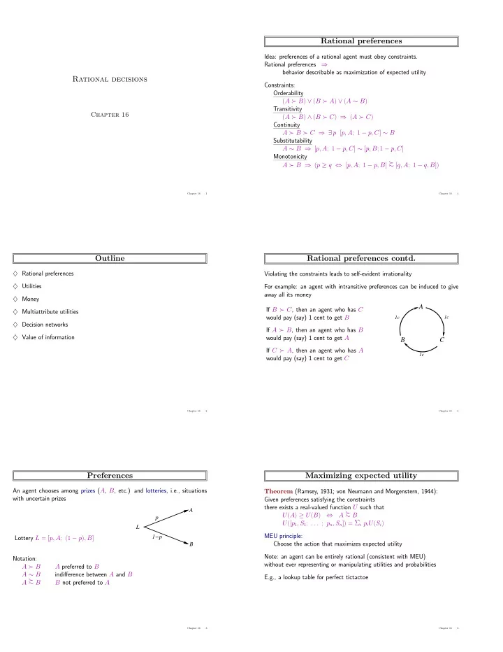♦ Rational preferences Violating the constraints leads to self-evident irrationality ♦ Utilities For example: an agent with intransitive preferences can be induced to give away all its money ♦ Money A If B ≻ C , then an agent who has C ♦ Multiattribute utilities 1c 1c would pay (say) 1 cent to get B ♦ Decision networks If A ≻ B , then an agent who has B ♦ Value of information would pay (say) 1 cent to get A B C If C ≻ A , then an agent who has A 1c would pay (say) 1 cent to get C Chapter 16 2 Chapter 16 5 Preferences Maximizing expected utility An agent chooses among prizes ( A , B , etc.) and lotteries, i.e., situations Theorem (Ramsey, 1931; von Neumann and Morgenstern, 1944): with uncertain prizes Given preferences satisfying the constraints there exists a real-valued function U such that A A ≻ U ( A ) ≥ U ( B ) ⇔ ∼ B p U ([ p 1 , S 1 ; . . . ; p n , S n ]) = Σ i p i U ( S i ) L 1−p MEU principle: Lottery L = [ p, A ; (1 − p ) , B ] B Choose the action that maximizes expected utility Note: an agent can be entirely rational (consistent with MEU) Notation: without ever representing or manipulating utilities and probabilities A ≻ B A preferred to B A ∼ B indifference between A and B E.g., a lookup table for perfect tictactoe A ≻ ∼ B B not preferred to A Chapter 16 3 Chapter 16 6

Utilities Student group utility Utilities map states to real numbers. Which numbers? For each x , adjust p until half the class votes for lottery (M=10,000) p Standard approach to assessment of human utilities: compare a given state A to a standard lottery L p that has 1.0 “best possible prize” u ⊤ with probability p 0.9 “worst possible catastrophe” u ⊥ with probability (1 − p ) 0.8 0.7 adjust lottery probability p until A ∼ L p 0.6 0.5 continue as before 0.999999 0.4 pay $30 0.3 ~ L 0.2 0.1 0.000001 instant death 0.0 $x 0 500 1000 2000 3000 4000 5000 6000 7000 8000 9000 10000 Chapter 16 7 Chapter 16 10 Utility scales Decision networks Add action nodes and utility nodes to belief networks Normalized utilities: u ⊤ = 1 . 0 , u ⊥ = 0 . 0 to enable rational decision making Micromorts: one-millionth chance of death useful for Russian roulette, paying to reduce product risks, etc. Airport Site QALYs: quality-adjusted life years useful for medical decisions involving substantial risk Air Traffic Deaths Note: behavior is invariant w.r.t. +ve linear transformation Litigation Noise U U ′ ( x ) = k 1 U ( x ) + k 2 where k 1 > 0 With deterministic prizes only (no lottery choices), only Construction Cost ordinal utility can be determined, i.e., total order on prizes Algorithm: For each value of action node compute expected value of utility node given action, evidence Return MEU action Chapter 16 8 Chapter 16 11 Money Multiattribute utility Money does not behave as a utility function How can we handle utility functions of many variables X 1 . . . X n ? E.g., what is U ( Deaths, Noise, Cost ) ? Given a lottery L with expected monetary value EMV ( L ) , usually U ( L ) < U ( EMV ( L )) , i.e., people are risk-averse How can complex utility functions be assessed from preference behaviour? Utility curve: for what probability p am I indifferent between a prize x and a lottery [ p, $ M ; (1 − p ) , $0] for large M ? Idea 1: identify conditions under which decisions can be made without com- plete identification of U ( x 1 , . . . , x n ) Typical empirical data, extrapolated with risk-prone behavior: Idea 2: identify various types of independence in preferences +U o o and derive consequent canonical forms for U ( x 1 , . . . , x n ) o o o o o o o o o o +$ −150,000 800,000 o o o Chapter 16 9 Chapter 16 12

Strict dominance Label the arcs + or – SocioEcon Typically define attributes such that U is monotonic in each Age GoodStudent Strict dominance: choice B strictly dominates choice A iff ExtraCar Mileage ∀ i X i ( B ) ≥ X i ( A ) (and hence U ( B ) ≥ U ( A ) ) RiskAversion VehicleYear This region X X 2 2 SeniorTrain dominates A B DrivingSkill MakeModel C B DrivingHist C Antilock A A DrivQuality HomeBase AntiTheft Airbag CarValue D Accident Ruggedness Theft X X 1 1 OwnDamage Deterministic attributes Uncertain attributes Cushioning OwnCost OtherCost MedicalCost LiabilityCost PropertyCost Strict dominance seldom holds in practice Chapter 16 13 Chapter 16 16 Stochastic dominance Label the arcs + or – SocioEcon 1.2 1 Age GoodStudent 1 0.8 ExtraCar Mileage 0.8 RiskAversion Probability Probability 0.6 VehicleYear 0.6 S1 S2 S1 0.4 SeniorTrain S2 0.4 + 0.2 DrivingSkill MakeModel 0.2 DrivingHist 0 0 -6 -5.5 -5 -4.5 -4 -3.5 -3 -2.5 -2 -6 -5.5 -5 -4.5 -4 -3.5 -3 -2.5 -2 Antilock Negative cost Negative cost DrivQuality HomeBase AntiTheft Airbag CarValue Distribution p 1 stochastically dominates distribution p 2 iff Accident � t � t Ruggedness ∀ t −∞ p 1 ( x ) dx ≤ −∞ p 2 ( t ) dt Theft OwnDamage If U is monotonic in x , then A 1 with outcome distribution p 1 Cushioning OwnCost OtherCost stochastically dominates A 2 with outcome distribution p 2 : � ∞ � ∞ −∞ p 1 ( x ) U ( x ) dx ≥ −∞ p 2 ( x ) U ( x ) dx MedicalCost LiabilityCost PropertyCost Multiattribute case: stochastic dominance on all attributes ⇒ optimal Chapter 16 14 Chapter 16 17 Stochastic dominance contd. Label the arcs + or – SocioEcon Stochastic dominance can often be determined without Age exact distributions using qualitative reasoning GoodStudent ExtraCar Mileage E.g., construction cost increases with distance from city RiskAversion VehicleYear S 1 is closer to the city than S 2 + SeniorTrain ⇒ S 1 stochastically dominates S 2 on cost + DrivingSkill MakeModel E.g., injury increases with collision speed DrivingHist Antilock Can annotate belief networks with stochastic dominance information: DrivQuality HomeBase AntiTheft Airbag CarValue X + → Y ( X positively influences Y ) means that − For every value z of Y ’s other parents Z Accident Ruggedness ∀ x 1 , x 2 x 1 ≥ x 2 ⇒ P ( Y | x 1 , z ) stochastically dominates P ( Y | x 2 , z ) Theft OwnDamage Cushioning OwnCost OtherCost MedicalCost LiabilityCost PropertyCost Chapter 16 15 Chapter 16 18