12. The Gradient and directional derivatives We have d f dx dy - - PDF document

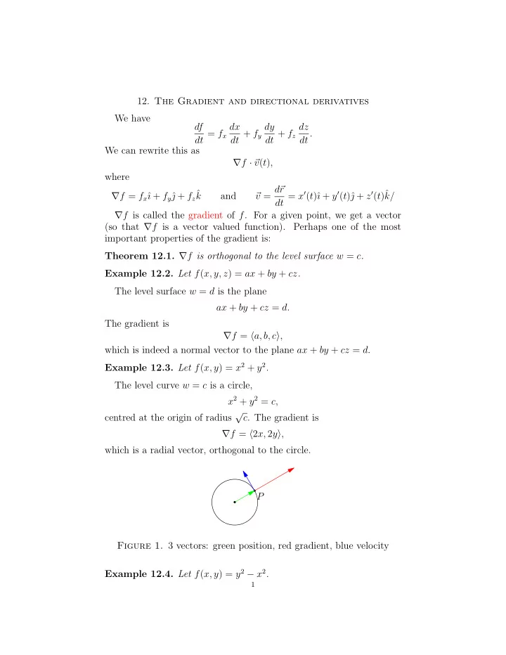
• 12. The Gradient and directional derivatives

We have d f dt = fx dx dt + fy dy dt + fz dz dt . We can rewrite this as ∇f · v(t), where ∇f = fxˆ ı + fyˆ  + fzˆ k and

• v = d

r dt = x′(t)ˆ ı + y′(t)ˆ  + z′(t)ˆ k/ ∇f is called the gradient of f. For a given point, we get a vector (so that ∇f is a vector valued function). Perhaps one of the most important properties of the gradient is: Theorem 12.1. ∇f is orthogonal to the level surface w = c. Example 12.2. Let f(x, y, z) = ax + by + cz. The level surface w = d is the plane ax + by + cz = d. The gradient is ∇f = a, b, c, which is indeed a normal vector to the plane ax + by + cz = d. Example 12.3. Let f(x, y) = x2 + y2. The level curve w = c is a circle, x2 + y2 = c, centred at the origin of radius √c. The gradient is ∇f = 2x, 2y, which is a radial vector, orthogonal to the circle. P Figure 1. 3 vectors: green position, red gradient, blue velocity Example 12.4. Let f(x, y) = y2 − x2.

1

The level curve is a hyperbola, y2 − x2 = c, with asymptotes y = x and y = −x. The gradient is ∇f = −2x, 2y. P Figure 2. Red gradient, blue tangent vector Proof of (??). Pick a curve r(t) contained in the level surface w = c. The velocity vector v = r′(t) is contained in the tangent plane. By the chain rule, 0 = dw dt = ∇f · v = 0, so that ∇f is perpendicular to every vector parallel to the tangent plane.

• We can use this to calculate the tangent plane. For example, consider

2x2 − y2 − z2 = 6. Let’s calculate the tangent plane to this surface at the point (x0, y0, z0) = (2, 1, 1). We have ∇f = 4x, −2y, −2z. At (x0, y0, z0) = (2, 1, 1), the gradient is 8, −2, −2, so that n = 4, −1, −1 is a normal vector to the tangent plane. It follows that the equation of the tangent plane is 0 = x − 2, y − 1, z − 1 · 4, −1, −1 so that 4x − y − z = 6, is the equation of the tangent plane. In this example, there are other ways to figure out an equation for the tangent plane. We could write z as a function of x and y, z =

• 2x2 − y2 − 6,

and find an equation for the tangent plane in the standard way. Beware that this is not always possible.

2

Suppose that we are at a point (x0, y0) in the plane and we move in a direction ˆ u = a, b. We can define the directional derivative in the direction ˆ

• u. Consider the line
• r(s) = x0, y0 + sa, b.

The velocity vector is ˆ u, which has unit length, so that the speed is

• ne. In other words,

r(s) is parametrised by arclength. dw ds

• ˆ

u

= lim

s→0

f(x0 + sa, y0 + sb) − f(x0, y0) ∆s . If ˆ u = ˆ ı, then the directional derivative is fx and if ˆ u = ˆ  then the directional derivative is fy. In general, if we slice the graph w = f(x, y) by vertical planes, the directional derivative is the slope of the resulting curve. dw ds

• ˆ

u

= ∇f · d r ds = ∇f · ˆ u. Question 12.5. Fix a vector v = c, d in the plane. Which unit vector ˆ u (1) maximises v · ˆ u? (2) minimises v · ˆ u? (3) When is v · ˆ u = 0? We know

• v · ˆ

u = | v||ˆ u| cos θ = | v| cos θ. | v| is fixed as v is fixed. So we want to (1) maximise cos θ, (2) minimise cos θ (3) and we want to know when cos θ = 0. This happens when (1) θ = 0, in which case cos θ = 1, (2) θ = π, in which case cos θ = −1, (3) and θ = π/2, in which case cos θ = 0. Geometrically the three cases correspond to: (1) ˆ u points in the same direction as v, (2) ˆ u points in the opposite direction, and (3) ˆ u is orthogonal to v. Now consider v = ∇f. The directional derivative is dw ds

• ˆ

u

= ∇f · ˆ u.

3

This is maximised when ˆ u points in the direction of ∇f. In other words, ∇f points in the direction of maximal increase, −∇f points in the direction of maximal decrease and it is orthogonal to the level

• curves. The magnitude |∇f| of the gradient is the directional derivative

in the direction of ∇f, it is the largest possible rate of change. In terms of someone climbing a mountain: ∇f points in the direction you need to go straight up the mountain, with magnitude the slope. −∇f points straight down and ∇f is orthogonal to the level curve, which is the direction which takes you around the mountain.

4