Constraint-based Testing Software Engineering Gordon Fraser - - PDF document

Constraint-based Testing

Software Engineering Gordon Fraser • Saarland University

Based on slides by Arnaud Gotlieb & Koushik Sen

But how to create the tests?

CC PC GACC CACC RACC CoC RICC GICC

• 1!+!H/

So many different test objectives...

Test Data Generation

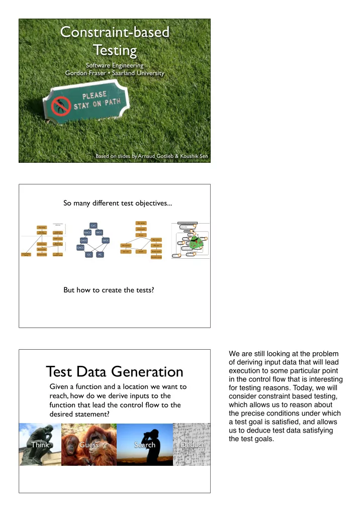
Given a function and a location we want to reach, how do we derive inputs to the function that lead the control flow to the desired statement? Deduce Think Search Guess

We are still looking at the problem

• f deriving input data that will lead

execution to some particular point in the control flow that is interesting for testing reasons. Today, we will consider constraint based testing, which allows us to reason about the precise conditions under which a test goal is satisfied, and allows us to deduce test data satisfying the test goals.

!" #$%&!'()*&!+!(,#-.(./ #$%&!'.)*&!+!.(#-.(./ 0,*!-1!+!2/ #$%&!#/ #!+!'()*&/ 03!4#!++!5657!"!! '.)*&!+!5!5/ 8! 9$0:(!4'()*&7!" ;&<( '.)*&!+!5=25/ &(*<&,!-1/ 8 >%:?( ;&<( 0,*!.0@0*A$0@$!+!B(CAD%:<(?E'466()*&7F/ 0,*!.0@0*A:-9!+!B(CAD%:<(?E'466()*&7F/ 03!4.0@0*A$0@$!++!GH!II!.0@0*A:-9!++!GH7!" ;&<(

• 1!+!H/

8 ;&<( (:?(!" '.)*&!+!HJ!'!.0@0*A$0@$!6!.0@0*A:-9/ 8 >%:?( 66.)*&/ 66()*&/ 8 >%:?( >%:?( !(:?(03!4#!++!5K57!" (:?( '.)*&!+!'()*&/ 8 0,*!#@0A.(#-.(4#$%&!'(,#-.(.L!#$%&!'.(#-.(.7 ! " # $ % & ' ( ) * +

A B C D E G F H I L M

Under which conditions do we reach this point? c has to be “+” *eptr has to be true

Constraint-based Testing

• Constraint generation

Extract a constraint system from the program and a testing objective

• Constraints on inputs

If inputs satisfy constraints, then testing objective will be satisfied

• Constraint solving:

Solve the constraint system to generate test data

• Static analysis aims at finding runtime

errors (e.g. division-by-zero, overflows, ...) at compile time

• CBT aims at finding functional faults (e.g. P

returns 3 while 2 was expected)

Looking at the control flow graph of the cgi_decode example, we see that in order to reach node E several conditions have to hold - conditions on variables that are altered during the program execution.

• Model-checking tools explore paths of

software models for proving properties

• CBT looks only for counter-examples
• Dynamic analysis approaches extract likely

invariants

• CBT exploits symbolic reasoning to find

counter-examples to given properties

Overview

• 1!+!H/

A B C D E G F H I L M

Program Constraint system

(a>b ∧ c = 2) ∨ (a>5 ∧ b>a) ∨ (a<b ∧ b<5 ∧ a > 0)

D

Test Goal

The ida of constraint based testing is to transform a program and a test goal for that program to a constraint system...

Overview

Constraint system

(a>b ∧ c = 2) ∨ (a>5 ∧ b>a) ∨ (a<b ∧ b<5 ∧ a > 0)

Constraint solver Test data

a = 1 b = 2 c = 3

Constraint Solving What is a constraint?

• A constraint is a condition that a solution

to an optimization problem must satisfy

• x > 5, y < 10
• a > b ∧ b > 10
• Constraint satisfaction:

Finding value assignments to variables such that constraints are satisfied

...and then use a constraint solver to automatically derive a solution to the constraint system - which is our test data. Relevant questions: Does the constraint system (CS) have a solution? Can we generate a solution to CS? Can we generate the best solution to CS?

Relevant Questions

• Does the constraint system (CS) have a solution?

To decide whether the testing objective is reachable or not

• Can we generate a solution to CS?

Test data generation

• Can we generate the best solution to CS?

Test data generation that optimizes a cost function

Constraint solving

• Computational domain, constraint language results from the

choice of programs and properties to be considered

• Booleans - Boolean formula (A&&B&&!C)||(...)
• Integers
• Bounded Integers
• Rationals
• Reals
• Floating-point numbers
• Decidability and

complexities

Boolean Formula Linear constraints Polynomial constraints Non-linear constraints Booleans 2-SAT in P 3-SAT is NP- complete 0-1 programming is NP-complete ? ? Bounded integers

• NP-complete

NP-complete NP-complete Integers

• Integer

programming is NP complete Undecidable Undecidable Rationals and reals

• Linear

programming in P Nonlinear programming is NP-complete Undecidable

The landscape of complexities for different domains (rows) and types

• f constraints (columns) looks

scary - in practice, however, we can handle anything involving non- linear constraints quite well using heuristics.

Decision procedures (best practices)

Boolean Formula Linear constraints Polynomial constraints Non-linear constraints Booleans Davis & Putnam (DPLL) Bounded integers Cooper’s procedure fir Oresburger algorith. Integers Constraint satisfaction Constraint satisfaction Constraint satisfaction Rationals and reals Simplex Fourier Elimination Groebner basis (Buchberger alg) Interval propagation

Constraint Satisfaction

• A constraint system involves a set of variables

V, a set of finite domains D, and a set of constraints C

• A solution is an assignment of

V to values in D that satisfies C

• A constraint system is unsatisfiable when it has no

solutions

• Constraint satisfaction involves 3 interleaved processes:

Constraint filtering Constraint propagation Variable labeling

Constraint filtering

• Given a single constraint, filter the domains
• f variables by removing inconsistent values
• Depends on a level of consistency to be

achieved Domain consistency - bound consistency - and many more

• Example:

X in {2,3,4,6,10}, Y in {1,2,3,4,6,8}, Z in {6}, X*Y=Z

Domain Consistency

For each value in Dx, find a support in Dz and Dy

X Z Y

{2,3,4,6,10} {6} {1,2,3,4,6,8} X*Y=Z

Bound Consistency

For each bound in Dx, find a support in Dz and Dy

X Z Y

{2,3,4,6,10} {6} {1,2,3,4,6,8} X*Y=Z

Constraint Propagation

• Propagates prunings throughout the constraint system
• Implemented as a fixpoint algorithm:

Agenda := C; while(!Agenda.isEmpty()) { c := POP(Agenda); D’ := narrow(c,D); if(D’ != D) Agenda := Agenda ∪ {c’ in C | vars(c’) ∩ vars(c)!=∅} D := D’ } return D’;

Domain consistency checks for each variable of a constraint for which of its values there is support in the values of the other variables. Bound consistency only reduces the domain bounds, and is therefore cheaper. After constraint filtering, the reduced value domains (result of function narrow in above source code) are propagated to other constraints that involve the same

• variables. This process is

implemented as a fixpoint algorithm that iterates until no more changes can be propagated.

Constraint Propagation

5 10 15 5 10 15

X, Y in 0..10, X*Y=6, X+Y=5

Constraint Propagation

3 6 9 12 15 3 6 9 12 15

X, Y in 0..10, X*Y=6, X+Y=5

Constraint Propagation

3 6 9 12 15 3 6 9 12 15

X, Y in 0..10, X*Y=6, X+Y=5

Constraint Propagation

3 6 9 12 15 3 6 9 12 15

X, Y in 0..10, X*Y=6, X+Y=5

Constraint Propagation

3 6 9 12 15 3 6 9 12 15

X, Y in 0..10, X*Y=6, X+Y=5 Fixpoint = X,Y in 2..3 called a hyper-box (in an n-dimensional space)

Variable Labeling

3 6 9 12 15 3 6 9 12 15

X, Y in 0..10, X*Y=6, X+Y=5 Select a value v from the domain of X and propagate X = v Solutions: {X=2, Y=3} {X=3, Y=2}

When heuristics for selecting values and variables are complete, labeling is a decision procedure for constraint satisfaction. But, it is also the costly part of it (NP- complete) while constraint filtering and propagation are polynomial in the number of constraints (and values in domains). Routinely in applications, constraint satisfaction handles thousands of constraints and variables

Selection Heuristics

• Leftmost

Select the leftmost variable in the list

• First-fail

Select the variable with the smallest domain

• Most-constrained

Select the var that has the most constraints suspended on it

• And many more

Variable Labeling

• When heuristics for selecting values and

variables are complete, labeling is a decision procedure for constraint satisfaction

• But, it is also the costly part of it (NP-

complete) while constraint filtering and propagation are polynomial in the number of constraints (and values in domains)

• Routinely in applications, constraint satisfaction

handles thousands of constraints and variables

Satisfiability Modulo Theory (SMT)

• To decide the satisfiability of formulas with

respect to decidable background theories . Φ ::= A | ¬Φ | Φ Φ | Φ Φ

• Numerous applications, including test data

generation

• Used in PEX, through Z3 the SMT
• solver of

Microsoft

Drop this slide

Satisfiability Modulo Theories (SMT)

• Example theories:
• R: theory of rationals

SR = {≤, +, -, 0, 1}

• L: theory of lists

SL = {=, hd, tl, nil, cons}

• E: theory of equality

SE: uninterpreted functions and predicate symbols

• Problem:

Is x ≤ y ∧ y ≤ x + hd(cons(0, nil)) ∧ P(h(x) - h(y)) ∧ ¬P(0) satisfiable in R.L.E ?

x ! y ! y ! x + hd(cons(0, nil)) ! P(h(x) - h(y)) ! ¬P(0)

v1

v3 v4 v2

x <= y y <= x+v1 v2 = v3-v4 x = y v2 = 0 !P(0) P(v2) v3 = h(x) v4 = h(y) v3 = v4 ⊥ v1=hd(cons(0,nil)) v1 = 0 R L E

SMT solving builds on the success

• f SAT solvers, and generalizes

boolean satisfiability to include theories. Z3 is one of the most powerful SMT solvers currently available. In this video, the authors of Z3 briefly describe constraint solving and demonstrate how to use a constraint solver via API calls. The video is available online at http:// channel9.msdn.com/posts/Peli/ The-Z3-Constraint-Solver/

Path-Oriented Testing Path-Oriented Generation

• Select one or several paths - Path selection
• Generate the path conditions - symbolic

evaluation techniques

• Solve the path conditions to generate test

data that activate the selected paths

• Useful for generating a test suite that covers

a given test criterion (all statements, all branches, all defs, all uses, ...)

Path Selection

double P(short x, short y) { short w = abs(y); double z = 1.0; while(w != 0) { z = z * x; w = w - 1; } if(y < 0) z = 1.0 / z; return z; }

The first step in a path oriented test generation technique is to select which path we want to execute in

• ur test case.

double P

double P(short x, short y) { short w = abs(y); double z = 1.0;

A

while(w != 0) {

B

z = z * x w = w - 1

C

if(y < 0)

D

z = 1.0 / z

E

return z; }

F

double P

double P(short x, short y) { short w = abs(y); double z = 1.0;

A

while(w != 0) {

B

z = z * x w = w - 1

C

if(y < 0)

D

z = 1.0 / z

E

return z; }

F

Statement coverage: A-B-C-B-D-E-F

double P

double P(short x, short y) { short w = abs(y); double z = 1.0;

A

while(w != 0) {

B

z = z * x w = w - 1

C

if(y < 0)

D

z = 1.0 / z

E

return z; }

F

Branch coverage: A-B-C-B-D-E-F A-B-D-F

double P

double P(short x, short y) { short w = abs(y); double z = 1.0;

A

while(w != 0) {

B

z = z * x w = w - 1

C

if(y < 0)

D

z = 1.0 / z

E

return z; }

F

LCSAJ: A-B-C-B-D-E-F A-B-D-F

double P

double P(short x, short y) { short w = abs(y); double z = 1.0;

A

while(w != 0) {

B

z = z * x w = w - 1

C

if(y < 0)

D

z = 1.0 / z

E

return z; }

F

Loop boundary: A-B-D-F A-B-C-B-D-F A-B-C-B-C-B-D-F

double P

double P(short x, short y) { short w = abs(y); double z = 1.0;

A

while(w != 0) {

B

z = z * x w = w - 1

C

if(y < 0)

D

z = 1.0 / z

E

return z; }

F

Boundary interior: A-B-D-F A-B-D-E-F A-B-C-B-D-F A-B-C-B-D-E-F A-B-D-B-C-B-D-F A-B-D-B-C-B-D-E-F

double P

double P(short x, short y) { short w = abs(y); double z = 1.0;

A

while(w != 0) {

B

z = z * x w = w - 1

C

if(y < 0)

D

z = 1.0 / z

E

return z; }

F

Path coverage: Unfeasible!

double P

double P(short x, short y) { short w = abs(y); double z = 1.0;

A

while(w != 0) {

B

z = z * x w = w - 1

C

if(y < 0)

D

z = 1.0 / z

E

return z; }

F

Reconsider: A-B-D-E-F

Infeasible! Determining whether an element is reachable or not is undecidable in the general case

Weyuker, 1979

Infeasible Paths

There is no guarantee that a path selected from the CFG is actually executable - paths can be infeasible, in which there is no input that would drive the execution through the chosen path.

Infeasible Paths

• Determining whether an element is

reachable or not is undecidable in the general case

• Infeasible paths are ubiquitous in imperative

programs

• Infeasible paths can be selected during the

path selection process

double P

double P(short x, short y) { short w = abs(y); double z = 1.0;

A

while(w != 0) {

B

z = z * x w = w - 1

C

if(y < 0)

D

z = 1.0 / z

E

return z; }

F

Def-use pair (z, A, E)

double P

double P(short x, short y) { short w = abs(y); double z = 1.0;

A

while(w >= 0) {

B

z = z * x w = w - 1

C

if(y < 0)

D

z = 1.0 / z

E

return z; }

F

Equivalent Mutants

We have encountered the infeasible path problem before - infeasible DU pairs are another example instance of the same problem. The equivalent mutant problem can also be reduced to the infeasible path problem.

Symbolic Evaluation

• Three path-oriented techniques:
• 1. Simple symbolic execution (forward and backward)
• 2. Dynamic symbolic execution
• 3. Global symbolic execution
• Exploits algebraic expressions over symbolic inputs to

represent internal states of variables

• Application in software testing, compiler optimization,

specialization, parallel computing, model-checking, program proving, etc.

double P

double P(short x, short y) { short w = abs(y); double z = 1.0; A while(w != 0) { B z = z * x w = w - 1 C if(y < 0) D z = 1.0 / z E return z; } F

• A: w := abs(Y); z := 1.0;
• B: abs(Y) != 0
• C: z := X; w := abs(Y) - 1;
• B: abs(Y) - 1 != 0
• C: z := X * X; w := abs(Y) - 2;
• B: abs(Y) - 2 = 0
• D: Y >= 0
• F: return (X*X);

Simple forward symbolic execution A-B-C-B-C-B-D-F with X, Y

Symbolic State

• <Path, State, Path Conditions>
• Path = ni - ... - nj is a path of a CFG
• State = {<v,φ>}v ∈

Var(P) where φ is an algebraic

expression over x

• Path Condition = ci ∧ .. ∧ cn where ck is a condition
• ver x
• x denotes symbolic variables associated to the inputs
• f program P and

Var(P) denotes internal variables

Given a path, we can derive constraints by symbolically executing the path either in a forward or backward fashion. During symbolic execution we maintain a symbolic state of the

• execution. If we encounter a

condition along the execution then the path conditions are updated, if we encounter assignments, then the state expressions are updated.

double P

double P(short x, short y) { short w = abs(y); double z = 1.0; A while(w != 0) { B z = z * x w = w - 1 C if(y < 0) D z = 1.0 / z E return z; } F

• A: w := abs(Y); z := 1.0;
• B: abs(Y) != 0
• C: z := X; w := abs(Y) - 1;
• B: abs(Y) - 1 != 0
• C: z := X * X; w := abs(Y) - 2;
• B: abs(Y) - 2 = 0
• D: Y >= 0
• F: return (X*X);

Simple forward symbolic execution A-B-C-B-C-B-D-F with X, Y

State

double P

double P(short x, short y) { short w = abs(y); double z = 1.0; A while(w != 0) { B z = z * x w = w - 1 C if(y < 0) D z = 1.0 / z E return z; } F

• A: w := abs(Y); z := 1.0;
• B: abs(Y) != 0
• C: z := X; w := abs(Y) - 1;
• B: abs(Y) - 1 != 0
• C: z := X * X; w := abs(Y) - 2;
• B: abs(Y) - 2 = 0
• D: Y >= 0
• F: return (X*X);

Simple forward symbolic execution A-B-C-B-C-B-D-F with X, Y

Path conditions

double P

double P(short x, short y) { short w = abs(y); double z = 1.0; A while(w != 0) { B z = z * x w = w - 1 C if(y < 0) D z = 1.0 / z E return z; } F

<A, {<z,⊥>, <w,⊥>}, true> <A-B-C-B, {<z,X>, <w,abs(Y)-1>}, abs(Y) != 0> <A-B-C-B-C-B-D-F, {<z,X2>, <w,abs(Y)-2>}, (abs(Y)!=0) ∧(abs(Y)!=1) ∧(abs(Y) =2) ∧(Y>=0)>

<Path, State, Path Conditions>

Computing Symbolic States

• <Path,State,PC> is computed by induction over

each statement of Path

• When the path conditions are unsatisfiable then

Path is infeasible

• Example: <A-B-D-E-F, {...}, abs(Y)=0 &&

Y<0 >

• Forward vs backward analysis:
• Forward: Interesting when states are needed
• Backward: Saves memory space as states remain

implicit

Example

Classify triangle by the length of the sides Equilateral Isosceles Scalene ((((((((234%"#)-*#"((((((((5$0$6-"-$((((((((((76#"-+-(

int triangle(int a, int b, int c) { if (a <= 0 || b <= 0 || c <= 0) { return 4; // invalid } if (! (a + b > c && a + c > b && b + c > a)) { return 4; // invalid } if (a == b && b == c) { return 1; // equilateral } if (a == b || b == c || a == c) { return 2; // isosceles } return 3; // scalene }

int triangle

int triangle(int a, int b, int c) {

A

if (! (a + b > c && a + c > b && b + c > a))

C

if (a <= 0 || b <= 0 || c <= 0) {

B

if (a == b && b == c) {

E

if (a == b || b == c || a == c) {

G

return 4;

D

return 3;

I

return 2;

J

return 1;

H

return 4;

F

A-B-C-E-H

• A: a :=X; b :=

Y; c := Z

• B: !(X<=0 ||

Y<=0 || Z<=0)

• C: (X+Y>Z && ...)
• E: X==Y &&

Y == Z

✔ ✔ ✔ ✔ ✔

Symbolic state at end: <A-B-C-E-H, {<a,X>, <b,Y>, <c,Z>}, ¬(X<=0 || Y<=0 || Z<=0)∧ (X+Y>Z ∧ ...) ∧ (X==Y ∧ Y == Z)>

• X>0 &&

Y>0 && Z>0 && X+Y>Z && X +Z>Y && Y+Z>X && X==Y && Y == Z

• Example, (1,1,1)

double P

double P(short x, short y) { short w = abs(y); double z = 1.0; A while(w != 0) { B z = z * x w = w - 1 C if(y < 0) D z = 1.0 / z E return z; } F

• F,D:

Y >= 0

• B:

Y>=0, w=0

• C:

Y>=0, w-1=0

• B:Y>=0,w-1=0,w!=0
• C:

Y>=0,w-2=0,w-1!=0

• B:

Y>=0,w-2=0,w-1!=0,w!=0

• A:

Y>=0, abs(Y)-2=0,abs (Y)-1=0,abs(Y)!=0 Backward Analysis A-B-C-B-C-B-D-F with X, Y Constraint system

The triangle example does not change the state along the execution, so symbolic execution reduces to collecting path conditions. In backward analysis, the state is not explicit as on forward execution (which means this needs less memory). We simply maintain the set of path conditions, and whenever we encounter a state update, we apply this update to the path conditions collected so far.

Example

Classify triangle by the length of the sides Equilateral Isosceles Scalene ((((((((234%"#)-*#"((((((((5$0$6-"-$((((((((((76#"-+-(

int triangle(int a, int b, int c) { if (a <= 0 || b <= 0 || c <= 0) { return 4; // invalid } if (! (a + b > c && a + c > b && b + c > a)) { return 4; // invalid } if (a == b && b == c) { return 1; // equilateral } if (a == b || b == c || a == c) { return 2; // isosceles } return 3; // scalene }

int triangle

int triangle(int a, int b, int c) {

A

if (! (a + b > c && a + c > b && b + c > a))

C

if (a <= 0 || b <= 0 || c <= 0) {

B

if (a == b && b == c) {

E

if (a == b || b == c || a == c) {

G

return 4;

D

return 3;

I

return 2;

J

return 1;

H

return 4;

F

A-B-C-E-G-J with X,Y,Z

• J,G: X ==

Y || Y == Z || X == Z

• E: ... && (X !=

Y || Y != Z)

• C: ... && (X+Y>Z &&

X+Z>Y && Y+Z>X)

• B: ... && (X>0 &&

Y>0 && Z>0)

✔ ✔ ✔ ✔ ✔ ✔

• (X ==

Y || Y == Z || X == Z) && (X != Y || Y != Z) && X+Y>Z && X+Z>Y && Y+Z>X && X>0 && Y>0 && Z>0

• Example, (1,1,1)

Implementing Symbolic Execution

• Transformation approach

Transform to program that operates only on symbolic values

• Instrumentation approach
• Customized runtime approach

Transformation Approach

• Transform the program to another

program that operates on symbolic values such that execution of the transformed program is equivalent to symbolic execution of the original program

Instrumentation Approach

• callback hooks are inserted in the program

such that symbolic execution is done in background during normal execution of program

• easy to implement for C

Customized runtime approach

• Customize the runtime (e.g. JVM) to

support symbolic execution

• Java PathFinder (NASA)
• Applicable to Java, .NET

Limitations

• Limited by the power of constraint solver

No non-linear or complex constraints

• Does not scale when number of paths is

large

• Source code or equivalent (Bytecode) is

required for precise symbolic execution

• Infeasible path problem

Goal-Oriented Testing Goal-oriented testing

• A three step process:
• 1. Generate a constraint model of the whole program
• 2. Choose a goal: point to be reached or property to

be refuted

• 3. Generate test data that respects the model and

satisfies the goal

• Useful for generating test data that reaches a single

testing objective (reach a statement or a branch, find a counter-example to a property, etc.)

A constraint model of imperative programs

• Viewing an assignment statement as a

relation requires to rename the variables

• i := i + 1 → i2 = i1 + 1
• Static Single Assignment (SSA) form or

single assignment language

Destructive assignment to variables makes it necessary to rename variables for representation in a logic system.

SSA form

• Each use of a variable refers to a single

definition

x := x + y; y := x - y; x := x - y; x1 := x0 + y0; y1 := x1 - y0; x2 := x1 - y1;

ϕ Functions

i := ...

2

i := ...

1

... := i + ...

3

i2 := ...

2

i1 := ...

1

i3 := ϕ(i1, i2) ... := i3 + ...

3

double P

double P(short x, short y) { short w = abs(y); double z = 1.0; A while(w != 0) { B z = z * x w = w - 1 C if(y < 0) D z = 1.0 / z E return z; } F

double P

double P(short x, short y) { short w1 = abs(y); double z1 = 1.0; A w3 = ϕ(w1,w2) z3 = ϕ(z1,z2) while(w3 != 0) { B z2 = z3 * x w2 = w3 - 1 C if(y < 0) D z4 = 1.0 / z3 E z5 := ϕ(z4,z3) return z5; } F

At join points in the control flow, we need to add phi functions that represent a choice of the values of the two branches. In an IF condition the phi function is simply added after the if and else branches, but for loops we need to add the phi function before loop condition.

From SSA to a Constraint System

Variable declaration Domain constraint Assignment, decision Arithmetical constraints {=, <, ...}

unsigned int i i ∈ 0...232-1 j2 = j1 * i i == j i < j j2 = j1 * i i = j i < j

From SSA to a Constraint System

Conditional (SSA) Iteration (SSA)

if D then C1 else C2 v3 := ϕ(v1, v2) (D ∧ C1 ∧ v3 = v1) ∨ (!D ∧ C2 ∧ v3 = v2) v3 := ϕ(v1, v2) while D do C v3 = v1 ∨ (D1 ∧ C1 ∧ !D2 ∧ v3=v2) ∨ ... double P

double P(short x, short y) { short w = abs(y); double z = 1.0; A while(w != 0) { B z = z * x w = w - 1 C if(y < 0) D z = 1.0 / z E return z; } F

double P

double P(short x, short y) { short w1 = abs(y); double z1 = 1.0; A w3 = ϕ(w1,w2) z3 = ϕ(z1,z2) while(w3 != 0) { B z2 = z3 * x w2 = w3 - 1 C if(y < 0) D z4 = 1.0 / z3 E z5 := ϕ(z4,z3) return z5; } F

Assignment and comparison have equal operations due to SSA. For conditionals and loops we need to get rid of the phi functions when converting to a constraint system. For a conditional this gives us a disjunction of the two possible

• utcomes of the condition (note

that v3 is assigned within this disjunction). Loops need to be unrolled. Conversion of the power function to SSA.

double P

double P(short x, short y) { short w1 = abs(y); double z1 = 1.0; A w3 = ϕ(w1,w2) z3 = ϕ(z1,z2) while(w3 != 0) { B z2 = z3 * x w2 = w3 - 1 C if(y < 0) D z4 = 1.0 / z3 E z5 := ϕ(z4,z3) return z5; } F double P(short x, short y) { short w1 = abs(y); double z1 = 1.0; A if(w1 != 0) { B if(y < 0) H z6 = 1.0 / z5 I z7 := ϕ(z5,z6) return z7; } J if(w2 != 0) { D z3 = z2 * x w3 = w2 - 1 E z2 = z1 * x w2 = w1 - 1 C z4 := ϕ(z2,z3) w4 := ϕ(w2,w3) F z5 := ϕ(z1,z4) w5 := ϕ(w1,w4) G double P(short x, short y) { short w1 = abs(y); double z1 = 1.0; A if(w1 != 0) { B if(y < 0) H z6 = 1.0 / z5 I z7 := ϕ(z5,z6) return z7; } J if(w2 != 0) { D z3 = z2 * x w3 = w2 - 1 E z2 = z1 * x w2 = w1 - 1 C z4 := ϕ(z2,z3) w4 := ϕ(w2,w3) F z5 := ϕ(z1,z4) w5 := ϕ(w1,w4) G

w1 = abs(y) ∧ z1 = 1.0 ∧ z2 = z1 * x ∧ w2 = w1 - 1 ∧ z3 = z2 * x ∧ w3 = w2 - 1 ∧ ((w2 =0 ∧ w4 = w2 ∧ z4 = z2) ∨ (w2 != 0 ∧ w4 = w3 ∧ z4 = z3)) ∧ ((w1 =0 ∧ z5 = z1 ∧ w5 = w1) ∨ (w1 != 0 ∧ z5 = z4 ∧ w5 = w4)) ∧ z6 = 1.0 / z5 ∧ ((y >= 0 ∧ z7 = z5) ∨ (y < 0 ∧ z6))

Test Objectives

t t t f t f Condition 1 Condition 2 Condition 3 Condition 4 Condition 4 ∧ Condition 2 ∧ Condition1

Loop unrolling (0,1, or 2 times) Resulting constraint system. To reach a certain point in the control flow the control dependencies need to be satisfied. For the constraint system, we add all the control dependent conditions.

double P(short x, short y) { short w1 = abs(y); double z1 = 1.0; A if(w1 != 0) { B if(y < 0) H z6 = 1.0 / z5 I z7 := ϕ(z5,z6) return z7; } J if(w2 != 0) { D z3 = z2 * x w3 = w2 - 1 E z2 = z1 * x w2 = w1 - 1 C z4 := ϕ(z2,z3) w4 := ϕ(w2,w3) F z5 := ϕ(z1,z4) w5 := ϕ(w1,w4) G

w1 != 0 ∧ w2 != 0

double P(short x, short y) { short w1 = abs(y); double z1 = 1.0; A if(w1 != 0) { B if(y < 0) H z6 = 1.0 / z5 I z7 := ϕ(z5,z6) return z7; } J if(w2 != 0) { D z3 = z2 * x w3 = w2 - 1 E z2 = z1 * x w2 = w1 - 1 C z4 := ϕ(z2,z3) w4 := ϕ(w2,w3) F z5 := ϕ(z1,z4) w5 := ϕ(w1,w4) G

w1 = abs(y) ∧ z1 = 1.0 ∧ z2 = z1 * x ∧ w2 = w1 - 1 ∧ z3 = z2 * x ∧ w3 = w2 - 1 ∧ ((w4 = w2 ∧ z4 = z2 ∧ w2 =0) ∨ (w4 = w3 ∧ z4 = z3 ∧ w2 != 0)) ∧ ((w1 = 0 ∧ z5 = z1 ∧ w5 = w1) ∨ (w1 != 0 ∧ z5 = z4 ∧ w5 = w4)) ∧ z6 = 1.0 / z5 ∧ ((y >= 0 ∧ z7 = z5) ∨ (y < 0 ∧ z7 = z6)) ∧ w1 != 0 ∧ w2 != 0

double P

double P(short x, short y) { short w = abs(y); double z = 1.0; A while(w != 0) { B z = z * x w = w - 1 C if(y < 0) D z = 1.0 / z E return z; } F

double P

double P(short x, short y) { short w1 = abs(y); double z1 = 1.0; A w3 = ϕ(w1,w2) z3 = ϕ(z1,z2) while(w3 != 0) { B z2 = z3 * x w2 = w3 - 1 C if(y < 0) D z4 = 1.0 / z3 E z5 := ϕ(z4,z3) return z5; } F

Example

Classify triangle by the length of the sides Equilateral Isosceles Scalene ((((((((234%"#)-*#"((((((((5$0$6-"-$((((((((((76#"-+-(

int triangle(int a, int b, int c) { if (a <= 0 || b <= 0 || c <= 0) { return 4; // invalid } if (! (a + b > c && a + c > b && b + c > a)) { return 4; // invalid } if (a == b && b == c) { return 1; // equilateral } if (a == b || b == c || a == c) { return 2; // isosceles } return 3; // scalene } int triangle(int a, int b, int c) { int r = 3; // scalene if (a <= 0 || b <= 0 || c <= 0) { r = 4; // invalid } else { if (!(a + b > c && a + c > b && b + c > a)) { r = 4; // invalid } else { if (a == b && b == c) { r = 1; // equilateral } else { if (a == b || b == c || a == c) { r = 2; // isosceles } } } } return r; }

int triangle(int a, int b, int c) { int r = 3; // scalene if (a <= 0 || b <= 0 || c <= 0) { r = 4; // invalid } if (!(a + b > c && a + c > b && b + c > a)) { r = 4; // invalid } if (a == b && b == c) { r = 1; // equilateral } else if (a == b || b == c || a == c) { r = 2; // isosceles } return r; }

int triangle(int a, int b, int c) { int r0 = 3; // scalene if (a <= 0 || b <= 0 || c <= 0) { r1 = 4; // invalid } else { if (!(a + b > c && a + c > b && b + c > a)) { r2 = 4; // invalid } else { if (a == b && b == c) { r3 = 1; // equilateral } else { if (a == b || b == c || a == c) { r4 = 2; // isosceles } r5 = ϕ(r4, r0); } r6 = ϕ(r5, r3); } r7 = ϕ(r6, r2); } r8 = ϕ(r7, r1); return r8; } int triangle(int a, int b, int c) { int r0 = 3; // scalene if (a <= 0 || b <= 0 || c <= 0) { r1 = 4; // invalid } else { if (!(a + b > c && a + c > b && b + c > a)) { r2 = 4; // invalid } else { if (a == b && b == c) { r3 = 1; // equilateral } else { if (a == b || b == c || a == c) { r4 = 2; // isosceles } r5 = ϕ(r4, r0); } r6 = ϕ(r5, r3); } r7 = ϕ(r6, r2); } r8 = ϕ(r7, r1); return r8; }

(r0 = 3) ∧ ((r1 = 4 ∧ r8 = r1 ∧ (a <=0 ∨ b <=0 ∨ c <=0)) ∨ (r8 = r7 ∧ !(a <=0 ∨ b <=0 ∨ c <=0))) ∧ ((r2 = 4 ∧ r7 = r2 ∧ (a+b<=c ∨ a+c<=b ∨ b+c<=a)) ∨ (r7 = r6 ∧ !(a+b<=c ∨ a+c<=b ∨ b+c<=a))) ∧ ((r3 = 1 ∧ r6 = r3 ∧ a = b ∧ b = c) ∨ (r6 = r5 ∧ !(a = b ∧ b = c))) ∧ ((r4 = 2 ∧ r5 = r4 ∧ (a=b ∨ b=c ∨ a=c)) ∨ (r5 = r0 ∧ !(a=b ∨ b=c ∨ a=c)))

int triangle(int a, int b, int c) { int r0 = 3; // scalene if (a <= 0 || b <= 0 || c <= 0) { r1 = 4; // invalid } else { if (!(a + b > c && a + c > b && b + c > a)) { r2 = 4; // invalid } else { if (a == b && b == c) { r3 = 1; // equilateral } else { if (a == b || b == c || a == c) { r4 = 2; // isosceles } r5 = ϕ(r4, r0); } r6 = ϕ(r5, r3); } r7 = ϕ(r6, r2); } r8 = ϕ(r7, r1); return r8; }