Constituintes maioritrios da gua do mar (S=35) Constituinte g kg -1 - - PowerPoint PPT Presentation

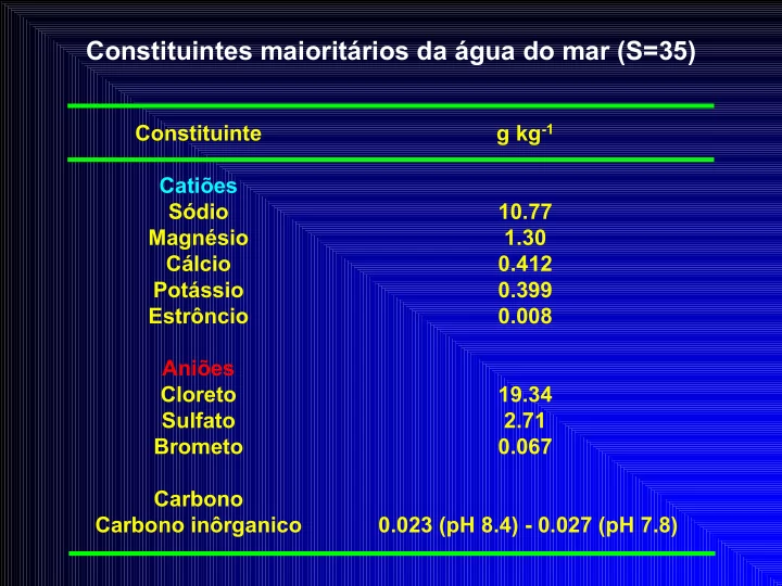
Constituintes maioritários da água do mar (S=35)

Constituinte g kg-1 Catiões Sódio 10.77 Magnésio 1.30 Cálcio 0.412 Potássio 0.399 Estrôncio 0.008 Aniões Cloreto 19.34 Sulfato 2.71 Brometo 0.067 Carbono Carbono inôrganico 0.023 (pH 8.4) - 0.027 (pH 7.8)

World ocean bathymetry World ocean bathymetry -

• NOAA

NOAA

Batimetria do Oceano Atlântico

Plataforma larga Crista média atlântica Plataforma estreita

North Atlantic Ridge North Atlantic Ridge

Bathymetry profile obtained by the Lamont-Doherty Earth Observatory at Columbia University http://imager.ldeo.columbia.edu/ridgembs/

Características gerais do oceano

Camada quente Província oceânica

Termoclina

Camada fria Província nerítica

Plataforma continental Declive continental z < 250m Planície abissal z ~4000m

T ~ 4oC S ~ 35

Pelagos Bentos

Polar easterlies Westerlies Subtropical highs Subtropical highs Westerlies Northeast trades Intertropical convergence zone Southeast trades 60o N 30o N 0o 30o S N

Major wind systems Major wind systems

• f the world
• f the world

60o S Polar easterlies S

General sub General sub-

• surface circulation of the World

surface circulation of the World Ocean Ocean

Norwegian Sea Iceland Faeroe Rise Sohm Abyssal Plain Demerara Abyssal Plain Brazil Basin Rio Grande Plateau Argentine Basin American Antartic Ridge Weddell Abyssal Plain Weddell Sea

A n t a r t i c B

• t

t

• m

W a t e r ( T m i n ) L a b r a d

• r

i n t e r m e d i a t e w a t e r ( S m i n ) NA Central Water SA Central Water Antartic intermediate water (Smin) North Atlantic Deep Water (Smax, Omax) Permanent t h e r m

• c

l i n e

60o N 40o N 20o N 0o 20o S 40o S 60o S 80o S

1000 2000 3000 4000 5000 6000

N

• r

w e g i a n

• verflow

S e a

Depth (m) Adapted from Dietrich et al., 1980 Adapted from Dietrich et al., 1980 -

• General Oceanography: An

General Oceanography: An Introduction Introduction

Coriolis Coriolis effect effect

• Coriolis parameter = 2Ω sin φ

Where:

Ω = rate of angular rotation of the earth φ = latitude

• Coriolis acceleration = 2Ωv sin φ

Where:

v = velocity

F=ma therefore:

• Coriolis force = 2Ωmv sin φ

Where:

m = mass

Ocean circulation Ocean circulation -

• 160 million years ago

160 million years ago

Upwelling areas Currents Continental drift

* http://earth.usc.edu/~stott/Catalina/Oceans.html

Ocean circulation Ocean circulation -

• 100 million years ago

100 million years ago

Continental drift Currents

http://earth.usc.edu/~stott/Catalina/Oceans.html

Ocean circulation Ocean circulation -

• 30 million years ago

30 million years ago

Continental drift Currents

http://earth.usc.edu/~stott/Catalina/Oceans.html

Global ocean Global ocean -

• surface gyres

surface gyres and temperatures and temperatures

Surface currents in the global ocean Surface currents in the global ocean

Cold current Cold current Warm current Warm current

Sea surface temperature Sea surface temperature -

• NOAA

NOAA

Data in oC - COADS monthly climatology dataset (1946-1989)

Global ocean surface temperature Global ocean surface temperature

December temperature (oC) December temperature (oC) -

• Data from NOAA

Data from NOAA

Global ocean surface temperature Global ocean surface temperature

July temperature (oC) July temperature (oC) -

• Data from NOAA

Data from NOAA

North Atlantic gyre North Atlantic gyre

Flows in Sverdrup (1 Sv = 10 Flows in Sverdrup (1 Sv = 106

6 m

m3

3 s

s-

• 1

1)

)

U.S.A. U.S.A.

Gulf stream Gulf stream current current

Temperature profile (oC) Temperature profile (oC)

Gulf stream current, showing ring formation Gulf stream current, showing ring formation

Circulação geral Circulação geral do Mar do Mar Mediterrâneo Mediterrâneo

40o N 45o N 5o W 0o W 5o E 10o E 15o E 20o E 25o E 30o E 35o E 1000m 2000m 3000m 4000m 28oC 20oC 12oC 4oC

Wind Wind-

• driven surface currents

driven surface currents

y x

Wind drag Water drag Coriolis

y x Wind drag y

Water drag Coriolis Water drag Coriolis

x Wind drag

Forces

y x

v

y x

v

45o y x

v Water velocity

Eckman Eckman spiral spiral -

• schematic representation

schematic representation

y 45o

z = 0 z = DE Wind

x

Horizontal projection of currents at 11 equally Horizontal projection of currents at 11 equally-

• spaced levels from the

spaced levels from the surface to bottom of the Eckman layer (D surface to bottom of the Eckman layer (DE

E)

)

Eckman Eckman spiral spiral -

• schematic representation

schematic representation

Wind Surface water Wind force Friction Direction of motion Wind force Direction

• f motion

Average flow 45o

Geostrophic Geostrophic balance balance

Continental mass

N

Water current Equator Coriolis force Wind stress

Balanced N-S wind stress and S-N coriolis force

E

Upwelling areas at western continental margin

S

Coastal Coastal upwelling upwelling -

• vertical section

vertical section

Front H H0 ρ1 ρ2 Ri D

H - Depth of water Ri - Rossby radius D - Distance to shore ρ1 - Density of upper water ρ2 - Density of lower water z - Depth

z

Mann & Lazier - Dynamics of Marine Ecosystems, Blackwell, 1991

Coastal Coastal upwelling upwelling -

• plan view

plan view

y (west) Front Coast x (south)

Mann & Lazier - Dynamics of Marine Ecosystems, Blackwell, 1991

Azores Front Azores Front

55oN 2000m 4000m 2000m 4000m 2000m 4000m 50o 45o 40o 35o 30o 25o 20o 70oW 60o 50o 40o 30o 20o 10o 5o

Data from Macedo et al, 1999

32.0 31.5 31.0 30.5 30.0 29.5 29.0 32.0 32.5 33.0 33.5 34.0 34.5 35.0 35.5 36.0 36.5 37.0 Depth (m)

Azores Front depth Azores Front depth contours contours

Latitude (º N)

350 300 250 200 150 100 50

Longitude (º W)

Data from Macedo et al, 1999

50 100 150 200 250 300 350 400 300 250 200 150 100 50

Depth( m)

Distance (km) 12 13 14 15 16 17 18 19 20 21 22 23 24 25 Temperature (ºC) North South

Temperature profile Temperature profile -

• Azores

Azores Front Front

Data from Macedo et al, 1999

Salinity profile Salinity profile -

• Azores

Azores Front Front

50 100 150 200 250 300 350 400 300 250 200 150 100 50 North

Distance (km)

Depth(m )

South

Salinity

36.8 36.7 36.6 36.5 36.4 36.3 36.2 36.1 36.0 35.9 35.8 35.7

Data from Macedo et al, 1999

Density profile Density profile -

• Azores

Azores Front Front

50 100 150 200 250 300 350 400 300 250 200 150 100 50

De pth( m )

North South

Density Distance (km)

24.2 24.4 24.6 24.8 25.0 25.2 25.4 25.6 25.8 26.0 26.2 26.4 26.6 26.8 27.0

Data from Macedo et al, 1999

Chlorophyll Chlorophyll a a profile profile -

• Azores

Azores Front Front

50 100 150 200 250 300 350 400

Distance (km)

300 250 200 150 100 50

Depth(m)

Chl a (mg m-3)

North South 0.26 0.24 0.22 0.20 0.18 0.16 0.14 0.12 0.10 0.08 0.06 0.04 0.02 0.00

Data from Macedo et al, 1999

Vertical profiles for temperature, chlorophyll a Vertical profiles for temperature, chlorophyll a and nitrate and nitrate -

• Azores Front

Azores Front

North South Depth (m)

Chlorophyll a (mg m-3) 0.42 Nitrate (mmol m-3) 0.5 1 1.5 2 2.5 3 3.5 4 0.5 1 1.5 2 2.5 3 3.5 4 Nitrate (mmol m-3)

Data from Macedo et al, 1999

252 240 228 216 204 192 180 168 156 144 132 120 108 96 84 72 60 48 36 24 12 NO3

• NO3
• T

T Chl a Chl a Temperature (ºC) 25 Temperature (ºC) 25 0.42 Chlorophyll a (mg m-3) 252 240 228 216 204 192 180 168 156 144 132 120 96 84 72 60 48 36 24 12 108

Tides and tide generating forces Tides and tide generating forces

To Sun Quadrature Syzygy North pole Sun

• Mass of the earth = 80X moon
• Mass of sun = 27 X 106 moon
• Sun-earth = 400X moon-earth

Tides and tide generating forces Tides and tide generating forces Model for a daily tide Model for a daily tide

24h Earth Tidal bulge Moon F = GMm r2

Tides and tide generating forces Tides and tide generating forces Model for a Model for a semi semi-

• diurnal

diurnal tide tide

Earth 29.5 days Moon Centre of rotation Is 1600km inside the earth (1/4 radius), and is the point about which the forces are balanced

Tides and tide generating forces Tides and tide generating forces Model for Model for tidal delay tidal delay

Earth Lunar orbit: 29.5 days 24h Moon Every day the moon moves approximately 360/30 degrees, i.e. 12o. The time on earth equivalent to 1 degree is 24 * 60 / 360 = 4 minutes, therefore the time lag is 12 * 4 = 48 minutes

Early tide gauges and prediction equipment Early tide gauges and prediction equipment

Tide gauge at Anchorage, Alaska Mechanical tide prediction machine

NOAA website

Mechanical tide prediction equipment Mechanical tide prediction equipment

NOAA website

Tides in the real ocean Tides in the real ocean

Types of constituents

• Semi-diurnal
• Diurnal
• Long-period
• Over 20 constituents may be required for accurate prediction

4 most important constituents Constituent Symbol Period Lunar semi-diurnal M2 12.42h Solar semi-diurnal S2 12.00h Luni-solar diurnal K1 23.93h Principal lunar diurnal O1 25.82h

Tides for March 2000 Tides for March 2000 -

• Tejo

Tejo Estuary Estuary

K1+O1 M2+S2 = 0.08 Data from OceanusTM - http://tejo.dcea.fct.unl.pt

Tides for March 2000 Tides for March 2000 -

• Dublin Bay

Dublin Bay

K1+O1 M2+S2 = 0.12 Data from OceanusTM - http://tejo.dcea.fct.unl.pt

Tides for March 2000 Tides for March 2000 -

• Do

Do-

• Son (Vietnam)

Son (Vietnam)

K1+O1 M2+S2 = 18.9 Data from OceanusTM - http://tejo.dcea.fct.unl.pt

Tides for March 2000 Tides for March 2000 -

• Manila

Manila

K1+O1 M2+S2 = 2.15 Data from OceanusTM - http://tejo.dcea.fct.unl.pt

Tides for March 2000 Tides for March 2000 -

• S. Francisco Bay
• S. Francisco Bay

K1+O1 M2+S2 = 0.90 Data from OceanusTM - http://tejo.dcea.fct.unl.pt

Bay of Bay of Fundy Fundy Extreme tidal range (>16m max) Extreme tidal range (>16m max)

Low tide High tide

Tagus Tagus estuary estuary -

• Space shuttle image

Space shuttle image

Caracterização geral Caracterização geral de um de um estuário estuário

Limite de baixa-mar Prisma de maré Q (m3 s-1)

Advecção & difusão

Maré Limite de preia-mar Rio Oceano

Distribuição longitudinal de salinidade

Rio 5 10 25 15 35 Oceano

Distribuição transversal de salinidade

Rio 5 10 25 15 35

Secção transversal homogénea

Oceano

Distribuição transversal de salinidade

Rio 5 10 25 15 35

Estratificação transversal

Oceano

Distribuição vertical de salinidade

Rio

Estratificação vertical

S Haloclina 25 35 5 10 15 Oceano Z (m) Coluna de água homogénea

Surface

10 20 km

GIS GIS -

• Salinity

Salinity

Tagus Tagus estuary estuary

Summer Winter

10 20 km

Surface

Summer Salinity (psu)

Bottom

Winter Salinity (psu)

10 20 km

Bottom

10 20 km

GIS GIS -

• Salinity

Salinity

Tagus Tagus estuary estuary -

• Summer

Summer

Surface

10 20 km

Bottom

10 20 km

Salinity (psu)

Surface - Bottom

10 20 km

Surface - Bottom Salinity (psu)

GIS GIS -

• Salinity

Salinity

Tagus Tagus estuary estuary -

• Winter

Winter

Surface

Salinity (psu)

10 20 km

Bottom

10 20 km

Surface - Bottom

10 20 km

Surface - Bottom Salinity (psu)

Salt wedge estuary

Classificação Classificação de de estuários estuários de Hansen & de Hansen & Rattray Rattray

δS S U U

s f

3b 1b 1a 3a 2b 2a Indice de estratificação

Hansen & Rattray, 1966 - Limnology & Oceanography 11, 319-326

100 10-1 10-2 102 101 Indice de circulação

Diagrama Diagrama de de diluição esquemático diluição esquemático

• Sódio

Sódio -

• Na+ (unidades arbitrárias)

Jusante Montante 12 6 Cl-

Diagrama Diagrama de de diluição esquemático diluição esquemático

• Cálcio

Cálcio -

• Ca2+ (unidades arbitrárias)

Cl- Jusante Montante 12 6

Diagrama Diagrama de de diluição esquemático diluição esquemático

• Sílica

Sílica ( (inverno inverno) ) -

• SiO2 (µmol l-1)

Jusante Montante 12 6 Cl-

Diagrama Diagrama de de diluição esquemático diluição esquemático

• Sílica

Sílica (primavera/ (primavera/verão verão) ) -

• SiO2 (µmol l-1)

Jusante Montante 12 6 Cl-

Diagrama Diagrama de de diluição esquemático diluição esquemático

• Nitrato

Nitrato (primavera/ (primavera/verão verão) ) -

• NO3
• (µmol l-1)

Jusante Montante 12 6 Cl-

Salinidade NO3

• (µmol l-1)

10 20 30 40 50 60 70 80 90 100 5 10 15 20 25 30 35 40

Montante

Diagrama Diagrama de de diluição diluição Estuário Estuário do do Tejo Tejo -

• Nitrato

Jusante

Nitrato

Jusante NO3

• (µmol l-1)

20 40 60 80 100 120 140 5 10 15 20 25 30 35 40

Montante

Diagrama Diagrama de de diluição diluição Estuário Estuário do do Guadiana Guadiana -

• Nitrato

Nitrato

Salinidade

Diagrama Diagrama de de diluição esquemático diluição esquemático

• Ferro

Ferro dissolvido dissolvido -

• Fe (mg l-1)

Jusante Montante 12 6 Cl-

Diagrama Diagrama de de diluição esquemático diluição esquemático

• Azoto amoniacal

Azoto amoniacal -

• NH4

+ (µmol l-1) Vila de Cima Vila de baixo

Jusante Montante 12 6 Cl-

Jusante Salinidade NH4

+ (µmol l-1)

5 10 15 20 25 30 5 10 15 20 25 30 35 40

Montante

Diagrama Diagrama de de diluição diluição Estuário Estuário do do Tejo Tejo -

• Azoto amoniacal

Azoto amoniacal

Jusante Salinidade NH4

+ (µmol l-1)

5 10 15 20 25 30 5 10 15 20 25 30 35 40

Montante

Diagrama Diagrama de de diluição diluição Estuário Estuário do do Sado Sado -

• Azoto amoniacal

Azoto amoniacal

Surface area to volume ratio (sinking rates) Surface area to volume ratio (sinking rates)

Sea surface

1mm cube surface area = 6mm2 volume = 1mm3 surface area = 6 volume Fall velocity W=2 g(D-d)r2 9 u 10mm cube surface area = 600mm2 volume = 1000mm3 surface area = 0.6 volume Relationship between forces Re=ud v

z (depth)

Reynolds number for different organisms

Organism Re Large whale (10 ms-1) 300 000 000 Tuna (10 m s -1) 30 000 000 Duck flying (20 ms -1) 300 000 Dragonfly (7 m s -1) 30 000 Copepod in a pulse of 20 cm s -1 300 Smallest flying insects 30 Invertebrate larva 0.3mm long at 1 mm s -1 0.3 Sea urchin sperm advancing the species at 0.3 mm s -1 0.03

Vogel, S, 1981 - Life in moving fluids. The physical biology of flow. Willard Grant Press, Boston, 352 pp.

Re = ud/v (2500 ~ threshold between laminar and turbulent flow) Re = 1.4 X 106 d 1.86 Relationship between length and swimming speed u (m s-1) = 1.4 X d 0.86 (kinematic viscosity = 10-6 m2 s-1)

Relação entre Relação entre o

• comprimento

comprimento e o e o número número de de Reynolds Reynolds

10 comprimentos s-1 1 comprimento s-1

Re = 1.4 X 106 d 1.86 Log número de Reynolds (Re) Log comprimento Comprimento

Mamíferos Peixes Anfípodes Zooplâncton Protozoários Fitoplâncton Bactérias Homem

• 6
• 4
• 2

2 4 6 8

• 6
• 4
• 2

2 1 µm 100 µm 1 m 1 cm 100 m

The length scale The length scale 1 1µ µm m-

• 100000km

100000km

Largest whale Mean depth

• f the ocean

Fish Zooplankton Internal Rossby radius Mixed- layer depth Diffusion limitation Phytoplankton Ocean basin Bacteria 1µm 1cm 1m 1km 1000km 10-6 10-4 10-2 100 102 104 106 108 Mann & Lazier, Dynamics of Marine Ecosystems, Blackwell 1991

Amostragem Euleriana

A B C D

Amostragem Euleriana Amostragem Euleriana ∫ V dt = h/3 (y0+4y1+2y2+...+4yn-1+yn)

Velocidade máxima de vazante Velocidade máxima de enchente t (s) V (ms-1) Estofo de BM e PM

200 400 600 Actual period

• 1.5
• 1
• 0.5

0.5 1 1.5 800 Sampling window

Actual period is double the apparent period

Apparent period

Sampling period and actual Sampling period and actual period period

Sampling frequency and event Sampling frequency and event

• ccurrence
• ccurrence

Event

12

Month

10 2 4 6 8

Sampling occasions

Event occurs every 3 months (seasonally), but appears to occur every six months