Computational challenges in experimental mathematics David H. Bailey - PowerPoint PPT Presentation

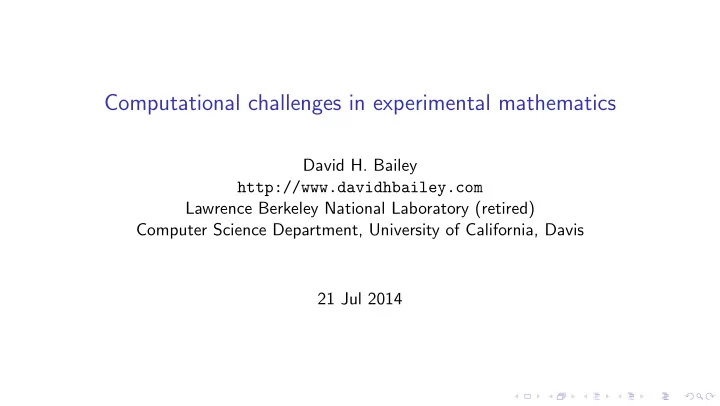
Computational challenges in experimental mathematics David H. Bailey http://www.davidhbailey.com Lawrence Berkeley National Laboratory (retired) Computer Science Department, University of California, Davis 21 Jul 2014

Numerical reproducibility in high-performance computing A December 2012 ICERM workshop on reproducibility in high-performance computing noted: Numerical round-off error and numerical differences are greatly magnified as computational simulations are scaled up to run on highly parallel systems. As a result, it is increasingly difficult to determine whether a code has been correctly ported to a new system, because computational results quickly diverge from standard benchmark cases. And it is doubly difficult for other researchers, using independently written codes and distinct computer systems, to reproduce published results. ◮ V. Stodden, D. H. Bailey, J. Borwein, R. J. LeVeque, W. Rider and W. Stein, “Setting the default to reproducible: Reproducibility in computational and experimental mathematics,” Jan 2013, available at http://www.davidhbailey.com/dhbpapers/icerm-report.pdf .

Analysis of collisions at the Large Hadron Collider ◮ The 2012 discovery of the Higgs boson at the ATLAS experiment in the LHC relied crucially on the ability to track charged particles with exquisite precision (10 microns over a 10m length) and high reliability (over 99% of roughly 1000 charged particles per collision correctly identified). ◮ Software: 5 millions line of C++ and python code, developed by roughly 2000 physicists and engineers over 15 years. ◮ Recently, in an attempt to speed up the calculation, researchers found that merely changing the underlying math library resulted in some collisions being missed or misidentified. Questions: ◮ How serious are these numerical difficulties? ◮ How can they be tracked down? ◮ How can the library be maintained, producing numerically reliable results?

U.C. Berkeley’s CORVETTE project and the “Precimonious” tool Objective: Develop software facilities to find and ameliorate numerical anomalies in large-scale computations: ◮ Facilities to test the level of numerical accuracy required for an application. ◮ Facilities to delimit the portions of code that are inaccurate. ◮ Facilities to search the space of possible code modifications. ◮ Facilities to repair numerical difficulties, including usage of high-precision arithmetic. ◮ Facilities to navigate through a hierarchy of precision levels (32-bit, 64-bit, 80-bit or higher as needed). The current version of this tool is known as “Precimonious.” ◮ C. Rubio-Gonzalez, C. Nguyen, H. D. Nguyen, J. Demmel, W. Kahan, K. Sen, D. H. Bailey and C. Iancu, “Precimonious: Tuning assistant for floating-point precision,” Proceedings of SC13 , 2013.

Innocuous example where high precision is required for reproducible results Problem: Find a polynomial to fit the data (1 , 1048579 , 16777489, 84941299 , 268501249 , 655751251 , 1360635409 , 2523398179, 4311748609) for arguments 0 , 1 , · · · , 8. The usual approach is to solve the linear system: � n � n � n  k =1 x n      n k =1 x k · · · a 0 k =1 y k k � n � n � n k =1 x n +1 � n k =1 x 2 k =1 x k · · · a 1 k =1 x k y k  k      k  = . . . . .  ...      . . . . .       . . . . .      � n � n � n k =1 x n +1 k =1 x 2 n k =1 x n k =1 x n � · · · a n k y k k k k A 64-bit computation (e.g., using Matlab, Linpack or LAPACK) fails to find the correct polynomial in this instance, even if one rounds results to nearest integer. However, if Linpack routines are converted to use double-double arithmetic (31-digit accuracy), the above computation quickly produces the correct polynomial: 1 + 1048577 x 4 + x 8 = 1 + (2 20 + 1) x 4 + x 8 f ( x ) =

Innocuous example, continued The result on the previous page can be obtained with double precision using Lagrange interpolation or the Demmel-Koev algorithm. But few scientists, outside of expert numerical analysts, are aware of these schemes. Besides, even these schemes fail for higher-degree problems. For example: (1 , 134217731 , 8589938753 , 97845255883 , 549772595201, 2097396156251 , 6264239146561 , 15804422886323 , 35253091827713, 71611233653971 , 135217729000001 , 240913322581691, 409688091758593) is generated by: 1 + 134217729 x 6 + x 12 = 1 + (2 27 + 1) x 6 + x 12 f ( x ) = Neither the Lagrange or Demmel-Koev algorithms get the right answer with double precision. In contrast, a straightforward Linpack scheme, implemented with double-double arithmetic, works fine for this and a wide range of similar problems.

Numerical analysis experts or high precision? 2010 U.C. Berkeley statistics: ◮ 870 seniors graduated in the Division of Mathematical and Physical Sciences (including Mathematics, Physics and Statistics), the College of Chemistry and the College of Engineering (including Computer Science). ◮ Many graduates in other fields (biology, economics, finance, medicine, psychology, etc.) will also do significant numerical computing in their professional work. ◮ 219 students enrolled in two sections of Math 128A, a one-semester introductory numerical analysis course required of applied math majors. ◮ Only 24 enrolled in Math 128B, a more advanced course. Conclusion: Only about 2% of Berkeley graduates that will do scientific computing in their career work have had advanced training in numerical analysis.

Other applications where high-precision arithmetic is useful or essential 1. Planetary orbit calculations (32 digits). 2. Supernova simulations (32–64 digits). 3. Certain components of climate modeling (32 digits). 4. Coulomb n-body atomic system simulations (32–120 digits). 5. Schrodinger solutions for lithium and helium atoms (32 digits). 6. Electromagnetic scattering theory (32–100 digits). 7. Scattering amplitudes of fundamental particles (32 digits). 8. Discrete dynamical systems (32 digits). 9. Theory of nonlinear oscillators (64 digits). 10. The Taylor algorithm for ODEs (100–600 digits). 11. Ising integrals from mathematical physics (100–1000 digits). 12. Problems in experimental mathematics (100–50,000 digits). ◮ D. H. Bailey, R. Barrio, and J. M. Borwein, “High precision computation: Mathematical physics and dynamics,” Applied Mathematics and Computation , vol. 218 (2012), pg. 10106–10121.

High-precision arithmetic in experimental mathematics Typical methodology: 1. Compute various mathematical entities (limits, infinite series sums, definite integrals, etc.) to high precision, typically 100–10,000 digits. 2. Use an integer relation algorithm such as “PSLQ” to recognize these numerical values in terms of well-known mathematical constants. 3. Devise formal mathematical proofs of the discovered relations. This approach has been extremely fruitful — literally thousands of new results. What’s more, this is a very accessible form of research — even undergraduates (if they have good programming skills) can make state-of-the-art contributions.

The PSLQ integer relation algorithm Let ( x n ) be a given vector of real numbers. An integer relation algorithm either finds integers ( a n ) such that a 1 x 1 + a 2 x 2 + · · · + a n x n = 0 (to within the “epsilon” of the arithmetic being used), or else finds bounds within which no relation can exist. The “PSLQ” algorithm of mathematician-sculptor Helaman Ferguson is the most widely used integer relation algorithm. Integer relation detection requires very high precision (at least n × d digits, where d is the size in digits of the largest a k ), both in the input data and in the operation of the algorithm. ◮ D. H. Bailey and D. J. Broadhurst, “Parallel integer relation detection: Techniques and applications,” Mathematics of Computation , vol. 70, no. 236 (Oct 2000), pg. 1719–1736.

PSLQ, continued ◮ PSLQ constructs a sequence of integer-valued matrices B n that reduce the vector y = x · B n , until either the relation is found (as one of the columns of matrix B n ), or else precision is exhausted. ◮ A relation is detected when the size of smallest entry of the y vector suddenly drops to roughly “epsilon” (i.e. 10 − p , where p is the number of digits of precision). ◮ The size of this drop can be viewed as a “confidence level” that the relation is not a numerical artifact: a drop of 20+ orders of magnitude almost always indicates a real relation. Efficient variants of PSLQ: ◮ 2-level and 3-level PSLQ perform almost all iterations with only double precision, updating full-precision arrays as needed. They are hundreds of times faster than the original PSLQ. ◮ Multi-pair PSLQ dramatically reduces the number of iterations required. It was designed for parallel systems, but runs faster even on 1 CPU.

Decrease of log 10(min | y i | ) in multipair PSLQ run