Common Features of Flow Networks Single Source Single Sink Flows - - PowerPoint PPT Presentation

▶

Apr 09, 2024 769 likes •899 views

Common Features of Flow Networks Single Source Single Sink Flows Simple setting: single source s and single sink t Network represented by a (directed) graph G = ( V , E ) every other node v is an internal node Each edge e has a

SLIDE 1

Common Features of Flow Networks

◮ Network represented by a (directed) graph G = (V , E) ◮ Each edge e has a capacity c(e) ≥ 0 that limits amount of

traffic on e

◮ Source(s) of traffic/data ◮ Sink(s) of traffic/data ◮ Traffic flows from sources to sinks ◮ Traffic is switched/interchanged at nodes

Flow: abstract term to indicate stuff (traffic/data/etc) that flows from sources to sinks.

Single Source Single Sink Flows

Simple setting:

◮ single source s and single sink t ◮ every other node v is an internal node ◮ flow originates at s and terminates at t

s 1 2 3 4 5 6 t 15 5 10 30 8 4 9 4 15 6 10 10 15 15 10

◮ Each edge e has a capacity c(e) ≥ 0 ◮ Source s ∈ V with no incoming edges ◮ Sink t ∈ V with no outgoing edges

Assumptions: All capacities are integer, and every vertex has at least one edge incident to it.

Definition of Flow

Two ways to define flows:

◮ edge based ◮ path based

They are essentially equivalent but have different uses. Edge based definition is more compact.

Edge Based Definition of Flow

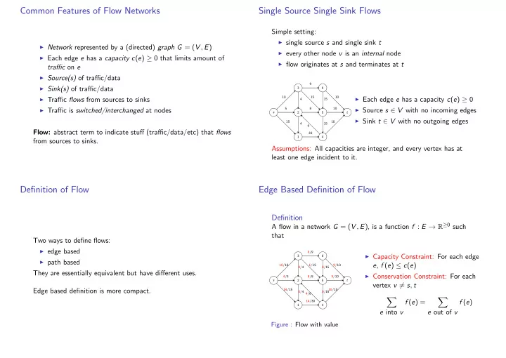
Definition

A flow in a network G = (V , E), is a function f : E → R≥0 such that

s 1 2 3 4 5 6 t 14/15 4/5 10/10 14/30 8/8 0/4 9/9 0/4 1/15 4/6 10/10 9/10 0/15 0/15 9/10

Figure : Flow with value

◮ Capacity Constraint: For each edge

e, f (e) ≤ c(e)

◮ Conservation Constraint: For each

vertex v = s, t

e into v

f (e) =

e out of v

f (e)

SLIDE 2

More Definitions and Notation

Notation

◮ The inflow into a vertex v is f in(v) =

e into v f (e) and the

utflow is f out(v) =

e out of v f (e)

◮ For a set of vertices A, f in(A) =

e into A f (e). Outflow f out(A) is defined analogously

Definition

For a network G = (V , E) with source s, the value of flow f is defined as v(f ) = f out(s)

A Path Based Definition of Flow

Intuition: flow goes from source s to sink t along a path. P: set of all paths from s to t. |P| can be exponential in n!

Definition

A flow in a network G = (V , E), is a function f : P → R≥0 such that

◮ Capacity Constraint: For each edge e, total flow on e is

≤ c(e).

p∈Pe

f (p) ≤ c(e)

◮ Conservation Constraint: No need! Automatic.

Value of flow:

p∈P f (p)

Path based flow implies Edge based flow

Lemma

Given a path based flow f : P → R≥0 there is an edge based flow f ′ : E → R≥0 of the same value.

Proof.

For each edge e define f ′(e) =

p:e∈p f (p).

Verify capacity and conservation constraints for f ′.

Edge based flow to Path based Flow

Flow Decomposition:

Lemma

Given an edge based flow f ′ : E → R≥0, there is a path based flow f : P → R≥0 of same value. Moreover, f assigns non-negative flow to at most m + n paths where |E| = m and |V | = n. Given f ′, the path based flow can be computed in O(mn) time.

Proof Idea.

◮ remove all edges with f ′(e) = 0 ◮ find a path p from s to t ◮ assign f (p) to be mine∈p f ′(e) ◮ reduce f ′(e) for all e ∈ p by f ′(e) ◮ repeat until no path from s to t

SLIDE 3

Edge vs Path based Definitions of Flow

Edge based flows:

◮ compact representation, only m values to be specified ◮ need to check flow conservation explicitly at each internal

node Path flows:

◮ in some applications, paths more natural ◮ not compact ◮ no need to check flow conservation constraints

Equivalence shows that we can go back and forth easily.

The Maximum-Flow Problem

Problem

Input A network G with capacity c and source s and sink t Goal Find flow of maximum value Question: Given a flow network, what is an upper bound on the maximum flow between source and sink?

Cuts

Definition

Given a flow network an s − t cut is a set of edges E ′ ⊂ E such that removing E ′ disconnects s from t: in other words there is no directed s → t path in E − E ′. The capacity of cut E ′ is

e∈E ′ c(e).

s 1 2 3 4 5 6 t 15 5 10 30 8 4 9 4 15 6 10 10 15 15 10

Caution: cut may leave t → s paths!

Minimum Cut

Definition

Given a flow network an s − t minimum cut is a cut E ′ of smallest capacity amongst all s − t cuts.

s 1 2 3 4 5 6 t 15 5 10 30 8 4 9 4 15 6 10 10 15 15 10

Observation: exponential number of s − t cuts and no “easy” algorithm to find a minimum cut.

SLIDE 4

The Minimum-Cut Problem

Problem

Input A network G with capacity c and source s and sink t Goal Find the capacity of a minimum s − t cut

Flows and Cuts

Lemma

For any s − t cut E ′, maximum s − t flow ≤ capacity of E ′.

Proof.

Formal proof easier with path based definition of flow. Suppose f : P → R≥0 is a max-flow. Every path p ∈ P contains an edge e ∈ E ′. Why? Assign each path p ∈ P to exactly on edge e ∈ E ′. Let Pe be paths assigned to e ∈ E ′. Then v(f ) =

p∈P

f (p) =

e∈E ′
p∈Pe

f (p) ≤

e∈E ′

c(e)

Flows and Cuts

Lemma

For any s − t cut E ′, maximum s − t flow ≤ capacity of E ′.

Corollary

Maximum s − t flow ≤ minimum s − t cut.

Max-Flow Min-Cut Theorem

Theorem

In any flow network the maximum s − t flow is equal to the minimum s − t cut. Can compute minimum-cut from maximum flow and vice-versa! Proof coming shortly. Many applications:

◮ optimization ◮ graph theory ◮ combinatorics

SLIDE 5

The Maximum-Flow Problem

Problem

Input A network G with capacity c and source s and sink t Goal Find flow of maximum value

Greedy Approach

s v u t 10/10 10/20 10/20 10/10 10/30

1. Begin with f (e) = 0 for each edge
2. Find a s-t path P with f (e) < c(e) for

every edge e ∈ P

3. Augment flow along this path
4. Repeat augmentation for as long as

possible.

Greedy Approach: Issues

s v u t 10 20/20 20/20 10 20/30

1. Begin with f (e) = 0 for each edge
2. Find a s-t path P with f (e) < c(e) for

every edge e ∈ P

3. Augment flow along this path
4. Repeat augmentation for as long as

possible. Need to “push-back” flow along edge (u, v)

Residual Graph

Definition

For a network G = (V , E) and flow f , the residual graph Gf = (V ′, E ′) of G with respect to f is

◮ V ′ = V ◮ Forward Edges: For each edge e ∈ E with f (e) < c(e), we

e ∈ E ′ with capacity c(e) − f (e)

◮ Backward Edges: For each edge e = (u, v) ∈ E with

f (e) > 0, we (v, u) ∈ E ′ with capacity f (e)

SLIDE 6

Residual Graph Example

s v u t 0/10 20/20 20/20 0/10 20/30

Figure : Flow in red edges

s v u t 10 20 20 10 20 10

Figure : Residual Graph

Ford-Fulkerson Algorithm

for every edge e, f(e) = 0 Gf is residual graph of G with respect to f while Gf has a simple s-t path let P be simple s-t path in Gf f = augment(f,P) Construct new residual graph Gf augment(f,P) let b be bottleneck capacity, i.e., min capacity of edges in P for each edge e in P if e is a forward edge f(e) = f(e) + b else (* e is a backward edge *) f(e) = f(e) - b return f

Properties about Augmentation

Lemma

If f is a flow and P is a simple s-t path in Gf , then f ′ = augment(f , P) is also a flow.

Lemma

At every stage of the Ford-Fulkerson algorithm, the flow values f (e) and the residual capacities in Gf are integers

Proof.

Initial flow and residual capacities are integers. Suppose lemma holds for j iterations. Then in j + 1st iteration, minimum capacity edge b is an integer, and so flow after augmentation is an integer.

Progress in Ford-Fulkerson

Proposition

Let f be a flow and f ′ be flow after one augmentation. Then v(f ) < v(f ′)

Proof.

Let P be an augmenting path, i.e., P is a simple s-t path in residual graph

◮ First edge e in P must leave s ◮ Original network G has no incoming edges to s; hence e is a

forward edge

◮ P is simple and so never returns to s ◮ Thus, value of flow increases by the flow on edge e

SLIDE 7

Termination Proof

Theorem

Let C = e out of s c(e). Ford-Fulkerson algorithm terminates after finding at most C augmenting paths

Proof.

The value of the flow increases by at least 1 after each

augmentation. Maximum value of flow is at most C.

Running time

◮ Number of iterations = O(C) ◮ Number of edges in Gf ≤ 2m ◮ Time to find augmenting path is O(n + m) ◮ Running time is O(C(n + m)) = O(mC)

Efficiency of Ford-Fulkerson

Running time = O(mC) is not polynomial. Can the upper bound be achieved?

s v u t C C C C 1 s v u t C C 1 C − 1 1 C − 1 1

Correctness of Ford-Fulkerson Augmenting Path Algorithm

Question: When the algorithm terminates, is the flow computed the maximum s − t flow? Proof idea: show a cut of value equal to the flow. Also shows that maximum flow is equal to minimum cut!

Definition

Given a flow network an s − t cut is a set of edges E ′ ⊂ E such that removing E ′ disconnects s from t: in other words there is no directed s → t path in E − E ′. The capacity of cut E ′ is

e∈E ′ c(e).

Cuts as Vertex Partitions

Let A ⊂ V such that

◮ s ∈ A, t ∈ A ◮ B = V − A and hence t ∈ B

Define (A, B) = {(u, v) ∈ E | u ∈ A, v ∈ B}

Claim

(A, B) is an s − t cut.

s 1 2 3 4 5 6 t 15 5 10 30 8 4 9 4 15 6 10 10 15 15 10

SLIDE 8

Cuts as Vertex Partitions

Lemma

Suppose E ′ is an s − t cut. Then there is a cut (A, B) such that (A, B) ⊆ E ′.

Proof.

E ′ is an s − t cut implies no path from s to t in (V , E − E ′). Let A be set of all nodes reachable by s in (V , E − E ′). By above, t ∈ A. And also (A, B) ⊆ E ′. Why?

Corollary

Every minimal s − t cut E ′ is a cut of the form (A, B).

Ford-Fulkerson Correctness

Lemma

If there is no s-t path in Gf then there is some cut (A, B) such that v(f ) = c(A, B)

Proof.

Let A be all vertices reachable from s in Gf ; B = V \ A

s u v′ u′ v t

◮ s ∈ A and t ∈ B. So (A, B) is an s-t

cut in G

◮ If e = (u, v) ∈ G with u ∈ A and

v ∈ B, then f (e) = c(e) because

therwise v is reachable from s

Lemma Proof Continued

Proof.

s u v′ u′ v t

◮ If e = (u′, v′) ∈ G with u′ ∈ B and

v′ ∈ A, then f (e) = 0 because

therwise u′ is reachable from s

◮ Thus,

v(f ) = f out(A) − f in(A) = c(A, B)

Ford-Fulkerson Correctness

Theorem

The flow returned by the algorithm is the maximum flow.

Proof.

◮ For any flow f and s-t cut (A, B), v(f ) ≤ c(A, B) ◮ For flow f ∗ returned by algorithm, v(f ∗) = c(A∗, B∗) for

some s-T cut (A∗, B∗)

◮ Hence, f ∗ is maximum

SLIDE 9

Max-Flow Min-Cut Theorem and Integrality of Flows

Theorem

For any network G, the value of a maximum s − t flow is equal to the capacity of the minimum s-t cut.

Theorem

For any network G with integer capacities, there is a maximum s − t flow that is integer valued.

Efficiency of Ford-Fulkerson

Running time = O(mC) is not polynomial. Can the upper bound be achieved?

s v u t C C C C 1 s v u t C C 1 C − 1 1 C − 1 1

Augmenting Paths with Large Bottleneck Capacity

◮ Pick augmenting paths with largest bottleneck capacity in

each iteration of Ford-Fulkerson

◮ How do we find path with largest bottleneck capacity?

◮ Assume we know ∆ the bottleneck capacity ◮ Remove all edges with residual capacity ≤ ∆ ◮ Check if there is a path from s to t ◮ Do binary search to find largest ∆ ◮ Running time: O(m log C)

Algorithm works in polynomial time but can devise a simpler algorithm.

Definition

Given graph G, s − t flow f and a parameter ∆, the graph Gf (∆) is the residual graph with all edges in Gf with residual capacity < ∆ removed.

Capacity Scaling Algorithm

for all edges e, f(e) = 0 ∆ = largest power of 2 smaller than maximum capacity edge in G while ∆ ≥ 1 while there is a simple s-t path in Gf (∆) let P be simple s-t path in Gf (∆) f = augment(f,P) update Gf (∆) ∆ = ∆/2

◮ Flows and residual capacities are always integral ◮ When ∆ = 1, Gf (∆) = Gf ; so on termination f is max-flow ◮ Outermost loop runs for at most ⌈log C⌉ + 1 ◮ Each augmentation increases flow by at least ∆

SLIDE 10

Running Time Analysis of Capacity Scaling Algorithm

◮ In each scaling phase there are at most 2m augmentations ◮ Each augmenting path can be found in O(m) time ◮ There are at most ⌈log C⌉ + 1 scaling phases ◮ Total time is O(m2 log C)

Paths in Gf (∆) and max-flows

Lemma

Let f be such that Gf (∆) does not have an s-t augmenting path. Then maximum flow is at most v(f ) + m∆.

Proof.

We will show that there is a cut (A, B) of capacity at most v(f ) + m∆

◮ Let A be all vertices reachable from s in Gf (∆), and let

B = V \ A; (A, B) is an s-t cut v(f ) =

e out of A f (e) − e into A f (e)

≥

e out of A[c(e) − ∆] − e into A ∆

=

e out of A c(e) − e out of A ∆ − e into A ∆

≥ c(A, B) − m∆

Augmentations per Scaling Phase

Proposition

There are at most 2m augmentation paths per scaling phase.

Proof.

◮ Let f be flow at end of previous scaling phase, i.e., with

scaling 2∆

◮ If f ∗ is max-flow, then v(f ∗) ≤ v(f ) + m(2∆) ◮ Since each augmentation in new phase increases flow by ∆,

there can be at most 2m augmentations to f

Removing Dependence on C

◮ [Edmonds-Karp, Dinitz] Picking augmenting paths with fewest

number of edges yields a O(m2n) algorithm, i.e., independent

f C!

◮ Further improvements can yield algorithms running in

O(mn log n), or O(n3)

SLIDE 11

Finding a Minimum Cut

Question: How do we find an actual minimum s − t cut? Proof gives the algorithm!

◮ Compute an s − t maximum flow f in G ◮ Obtain the residual graph Gf ◮ Find the nodes A reachable from s in Gf ◮ Output the cut (A, B) = {(u, v) | u ∈ A, v ∈ B}