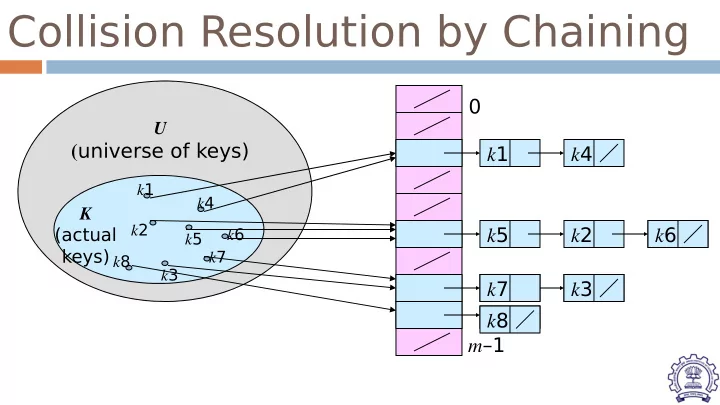
Collision Resolution by Chaining 0 U ( universe of keys) k 1 k 4 k - - PowerPoint PPT Presentation

k2

Collision Resolution by Chaining

m–1

U

(universe of keys)

K (actual keys)

k1 k2 k3 k5 k4 k6 k7 k8

k1 k4 k5 k6 k7 k3 k8

Expected Cost of an Search

Theorem: An unsuccessful search takes expected time Θ(1+α). Theorem: A successful search takes expected time Θ(1+α).

Proof Idea: T

• search unsuccessfully for any key k, need to

search to the end of the list T[h(k)], and E[T[h(k)]] = α. Proof Idea: T

• search successfully, calculate probability that

key i collides with j and j was inserted before i. Average over all n keys.

3

Open Addressing

 If we have enough contiguous memory to store all the keys (m >

n) ⇒ store the keys in the table itself

 No need to use linked lists anymore  Basic idea: 

Insertion: if a slot is full, try another one, until you find an empty one



Search: follow the same sequence of probes



Deletion: more difficult, we will see later

 Search time depends on the length of the probe sequence!

Linear Probing – Get And Put

 Let m = 17 and h(k) = k % 17.

4 8 12 16

• Put in pairs whose keys are 6, 12, 34,

29, 28, 11, 23, 7, 0, 33, 30, 45

6 1 2 2 9 34 2 8 1 1 23 7 3 3 3 45

Useful way to think about probing

 Let h(k) be the hash function used  When a collision occurs, try a different table cell.

 Try in succession h0(x), h1(x), h2(x), ...  hi(x) = (h(x) + f(i)) mod m, with f(0) = 0

 i = 0, 1, 2, …, m-1

 Function f is the collision resolution strategy.

 With linear probing, f is a linear function of i,

typically, f(i) = i

CENG 213 Data Structures

Clustering Problem

 As long as table is big enough, a free cell can

always be found, but the time to do so can get quite large.

 Worse, even if the table is relatively empty,

blocks of occupied cells start forming.

 This effect is known as primary clustering.  Any key that hashes into the cluster will require

several attempts to resolve the collision, and then it will add to the cluster.

Revisit the Example

 Let m = 17 and h(k) = k % 17.

4 8 12 16

• Put in pairs whose keys are 6, 12, 34,

29, 28, 11, 23, 7, 0, 33, 30

• Consider what happens when we insert

45

6 1 2 2 9 34 2 8 1 1 23 7 3 3 3

7

Performance Of Linear Probing

 Worst-case get/put time is O(n), where n is the number of pairs in the table.  This happens when all pairs are in the same cluster.

4 8 12 16 6 12 29 34 28 11 23 7 33 30 45

Expected Performance

 alpha = loading density = number of pairs/slots = n/m.

• alpha = 12/17.

 Sn = expected number of buckets examined in a successful search when n is

large

 Un = expected number of buckets examined in a unsuccessful search when n

is large

 Time to put governed by Un.

4 8 12 16 6 12 29 34 28 11 23 7 33 30 45

Expected Performance

 Sn ~ ½(1 + 1/(1 – alpha))  Un ~ ½(1 + 1/(1 – alpha)2)  Note that 0 <= alpha <= 1

Alpha <= 0.75 is recommended.

alpha S

n

Un 0.50 1.5 2.5 0.75 2.5 8.5 0.90 5.5 50.5

Hash T able Design

 Performance requirements are given, determine maximum permissible loading

density.

 We want a successful search to make no more than 10 compares (expected).

• Sn ~ ½(1 + 1/(1 – alpha))
• alpha <= 18/19

 We want an unsuccessful search to make no more than 13 compares (expected).

• Un ~ ½(1 + 1/(1 – alpha)2)
• alpha <= 4/5

 So alpha <= min{18/19, 4/5} = 4/5.

Quadratic Probing

 Quadratic Probing eliminates primary clustering problem of linear

probing.

 Collision function is quadratic.  The popular choice is f(i) = i2.  If the hash function evaluates to h and a search in cell h is

inconclusive, we try cells h + 12, h+22, … h + i2.

 i.e. It examines cells 1,4,9 and so on away from the original probe.  Remember that subsequent probe points are a quadratic

number of positions from the original probe point.

Homework

 Let m = 17 and h(k) = k % 17.  Put in pairs whose keys are 6, 12, 34, 29, 28, 11, 23, 7,

0, 33, 30, 45

 Homework:

 Find average length of probe if linear probe is used  Perform quadratic probing with f(i) = i2

 List the positions of all the keys

 Find the average length of probe if quadratic probe is used

Hash T able Design

 Dynamic resizing of table.

• Whenever loading density exceeds threshold (4/5

in our example), rehash into a table of approximately twice the current size.

Nature Lover’s View of A Tree

root branches leaves

Computer Scientist’s View

branches leaves root nodes

Linear Lists And Trees

 Linear lists are useful for serially ordered data.  (e0, e1, e2, …, en-1)  Days of week.  Months in a year.  Students in this class.  Trees are useful for hierarchically ordered data.  Employees of a corporation.

 President, vice presidents, managers, and so on.

 Java’s classes.

 Object is at the top of the hierarchy.  Subclasses of Object are next, and so on.

Hierarchical Data And Trees

 The element at the top of the hierarchy is the root.  Elements next in the hierarchy are the children of

the root.

 Elements next in the hierarchy are the and children

• f the root, and so on.

 Elements that have no children are leaves.

Definition

 A tree t is a finite nonempty set of elements.  One of these elements is called the root.  The remaining elements, if any, are

partitioned into trees, which are called the subtrees of t.

Caution

 Some texts start level numbers at 0 rather than at 1.  Root is at level 0.  Its children are at level 1.  The grand children of the root are at level 2.  And so on.  We shall number levels with the root at level 1.

height = depth = number of levels

Level 3 Object Number Throwable OutputStream Integer Double Exception FileOutputStream RuntimeException Level 4

Node Degree = Number Of Children

Object Number Throwable OutputStream Integer Double Exception FileOutputStream RuntimeException 3 2 1 1 1

Tree Degree = Max Node Degree

Object Number Throwable OutputStream Integer Double Exception FileOutputStream RuntimeException

3 2 1 1 1

Degree of tree = 3.

Binary Tree

 Finite (possibly empty) collection of elements.  A nonempty binary tree has a root element.  The remaining elements (if any) are partitioned into two

binary trees.

 These are called the left and right subtrees of the binary tree.

Differences Between A Tree & A Binary Tree

 No node in a binary tree may have a

degree more than 2, whereas there is no limit on the degree of a node in a tree.

 A binary tree may be empty; a tree

cannot be empty.

Differences Between A Tree & A Binary Tree

 The subtrees of a binary tree are ordered;

those of a tree are not ordered.

a b a b

• Are different when viewed as binary trees.
• Are the same when viewed as trees.

Arithmetic Expressions

 (a + b) * (c + d) + e – f/g*h + 3.25  Expressions comprise three kinds of entities.

 Operators (+, -, /, *).  Operands (a, b, c, d, e, f, g, h, 3.25, (a + b), (c + d), etc.).  Delimiters ((, )).

Binary Tree Properties & Representation

Minimum Number Of Nodes

 Minimum number of nodes in a binary tree whose height is h.  At least one node at each of first h levels.

minimum number of nodes is h

Maximum Number Of Nodes

 All possible nodes at first h levels are present.

Maximum number of nodes = 1 + 2 + 4 + 8 + … + 2h-1 = 2h - 1

Number Of Nodes & Height

 Let n be the number of nodes in a binary tree

whose height is h.

 h <= n <= 2h – 1  log2(n+1) <= h <= n

Full Binary Tree

 A full binary tree of a given height h has 2h – 1 nodes.

Height 4 full binary tree.

Numbering Nodes In A Full Binary Tree

 Number the nodes 1 through 2h – 1.  Number by levels from top to bottom.  Within a level number from left to right.

1 2 3 4 5 6 7 8 9 10 11 12 13 14 15