Classifica4on Binary classifica,on Given a set of examples ( x i , - - PDF document

classifica4on
SMART_READER_LITE
LIVE PREVIEW

Classifica4on Binary classifica,on Given a set of examples ( x i , - - PDF document

4/17/09 CSCI1950Z Computa4onal Methods for Biology Lecture 18 Ben Raphael April 8, 2009 hIp://cs.brown.edu/courses/csci1950z/ Classifica4on Binary classifica,on Given a set of examples ( x i , y i ) , where y i = + 1, from unknown


slide-1
SLIDE 1

4/17/09 1

CSCI1950‐Z Computa4onal Methods for Biology Lecture 18

Ben Raphael April 8, 2009

hIp://cs.brown.edu/courses/csci1950‐z/
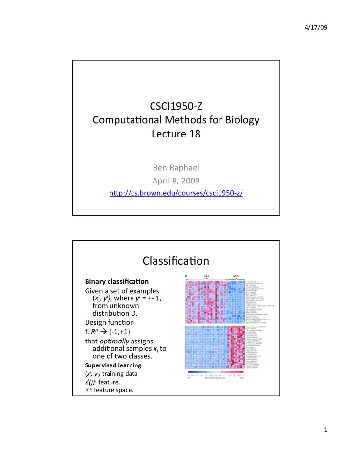
Classifica4on

Binary classifica,on Given a set of examples (xi, yi), where yi = +‐ 1, from unknown distribu4on D. Design func4on f: Rn  {‐1,+1} that op+mally assigns addi4onal samples xi to

  • ne of two classes.

Supervised learning (xi, yi) training data xi(j): feature. Rn: feature space.

slide-2
SLIDE 2

4/17/09 2

Dimensionality Reduc4on

Genomic data (e.g. gene expression) o[en high‐ dimensional (n > 5000), but rela4vely few samples available. Reduce dimensionality of data (lower dimensional subspace) to improve performance of the classifier by:

  • Removing features that do not contribute to the

classifica4on and may introduce noise.

  • Reducing opportuni4es for overfi]ng.
  • Improving 4me/memory efficiency in algorithms

for learning and classifica4on.

Feature Construc4on

Common method: Principal components analysis. [Whiteboard]

l features n features Linear/nonlinear transforma4on

slide-3
SLIDE 3

4/17/09 3

PCA and Clustering

Yeung and Ruzzo (Bioinforma4cs 2001)

Yeast gene expression data (477 genes) clustered into 7 clusters. First two principal components contain ≈89% of varia4on in data.

PCA and Clustering

Exon and junc4on microarrays detect widespread mouse strain‐ and sex‐bias expression differences. (Su et al. BMC Genomics 2008)

slide-4
SLIDE 4

4/17/09 4

Feature Selec4on

  • Selec4ng l << n

features that are informa(ve for classifica4on.

  • Gene expression:

subset of genes.

Feature Selec4on

Informa4ve features: Use a measure of associa4on between xi and yi.

  • Correla4on:
  • Chi‐square (con4ngency table)
  • Fischer criterion:

(xi)+ are elements in + class.

  • t‐test sta4s4c
  • Mutual informa4on
  • TNoM score (previous lecture) [Whiteboard]

rxiyi = m

k=1(xi k − xi)(yi k − yi)

(m − 1)sxisyi

F(xi) = |(xi)+ − (xi)−|2 s2

(xi)+ + s2 (xi)−

slide-5
SLIDE 5

4/17/09 5

Feature Selec4on Results

Colon Leukemia

Feature Selec4on Results

Top scoring genes (TNoM < 14) in colon dataset.

slide-6
SLIDE 6

4/17/09 6

Assessing Performance

Feature Selec4on (e.g. TNoM) Build Classifier Test

Cross‐valida4on WRONG

Assessing Performance

Must assess performance of both steps together!

Feature Selec4on (e.g. TNoM) Build Classifier Test

Cross‐valida4on

slide-7
SLIDE 7

4/17/09 7

Gene Selec4on Results

Predictors of Breast Cancer Prognosis

  • 70 gene signature to

predict breast cancer pa4ents with metastasis within 5 years (van de Vijver et al. NEJM 2002, van’t Veer et al. Nature 2002)

  • Now an FDA

approved test: Mammaprint

slide-8
SLIDE 8

4/17/09 8

Predictors of Breast Cancer Prognosis

n = 25000 genes 98 tumors. Hierarchical clustering: genes and samples n = 5000 differen+ally expressed genes

>2 fold change (and p<0.01) in >4 tumors

Step 1: Clustering

Predictors of Breast Cancer Prognosis

n = 5000 genes differen4ally expressed genes in 78 (sporadic lymph‐node nega4ve) tumors. Choose 231 genes with |ρ(xi, yi)| > 0.3. Rank genes by ρ(xi, yi). Compute correla4on coefficient ρ(xi, yi) Between each gene and prognosis. Step 2: Classifica4on

slide-9
SLIDE 9

4/17/09 9

Predictors of Breast Cancer Prognosis

n = 5000 genes differen4ally expressed genes in 78 (sporadic lymph‐node nega4ve) tumors. Choose 231 genes with |ρ(xi, yi)| > 0.3. Rank genes by ρ(xi, yi). Compute correla4on coefficient ρ(xi, yi) Between each gene and prognosis. Step 2: Classifica4on

Predictors of Breast Cancer Prognosis

Leave‐out one sample x. Let R = top 5 genes in list of 231. Compute correla4on coefficients ρ(μ(xR+), xR) and ρ(μ(xR‐), xR), where μ(xR+) is mean vector of genes in + class in R . Step 3: Build a classifier Assign to best class. Add 5 genes to R un4l performance does not improve.

slide-10
SLIDE 10

4/17/09 10

Predictors of Breast Cancer Prognosis

  • 70 gene classifier
  • 65/78 (83%) of pa4ents

predicted correctly.

– 5 poor and 8 good incorrectly assigned.

  • Changing threshold gave

3 poor and 12 good incorrectly assigned.

Discussion

  • Cross‐valida4on done a[er

feature selec4on!

– Also fixed this problem.

  • Resul4ng 70 gene signature is

not unique (Ein‐Dor et. al 2005: see notes)

  • Drawing biological

conclusions from the output

  • f a “black box” predic4on

algorithm is not wise.

– Correla4on vs. causality.

slide-11
SLIDE 11

4/17/09 11

Results: Class Discovery with TNoM (ben‐Dor, Friedman, Yakhini, 2001)

  • Find op4mal labeling L.

– Solu4on: use heuris4c search

  • Find mul4ple (subop4mal) labelings

– Solu4on: Peeling: remove previously used genes from set.

Results: Class Discovery with TNoM

(ben‐Dor, Friedman, Yakhini, 2001)

Leukemia (Golub et al. 1999): 72 expression profiles. 25 AML, 47 ALL. 7129 genes Lymphoma (Alizadeh et al.): 96 expression profiles, 46 Diffuse large B‐cell lymphoma (DLBCL) 50 from 8 different 4ssues. Lymphoma‐DLBCL: subset of 46 of above.

slide-12
SLIDE 12

4/17/09 12

TNoM Results

(ben‐Dor, Friedman, Yakhini, 2001)

% survival 24 pa4ents with low clinical risk. 40 pa4ents years