Chapter 6: Numerical Methods 6.1 Euler Method Basic Idea y ODE: y - - PowerPoint PPT Presentation

Chapter 6: Numerical Methods

6.1 Euler Method Basic Idea

• ODE: y′ = f(t, y)
• Assume y(t) is known
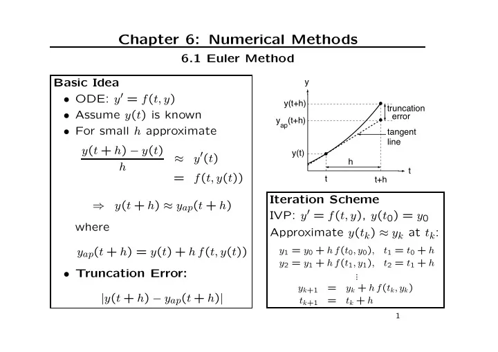
• For small h approximate

y(t + h) − y(t) h ≈ y′(t) = f(t, y(t)) ⇒ y(t + h) ≈ yap(t + h) where yap(t + h) = y(t) + h f(t, y(t))

• Truncation Error:

|y(t + h) − yap(t + h)|

t y(t) t+h y(t+h) h yap(t+h) t y truncation error tangent line

Iteration Scheme IVP: y′ = f(t, y), y(t0) = y0 Approximate y(tk) ≈ yk at tk:

y1 = y0 + h f(t0, y0), t1 = t0 + h y2 = y1 + h f(t1, y1), t2 = t1 + h . . . yk+1 = yk + h f(tk, yk) tk+1 = tk + h

1

Ex: Approximate the solution to y′ = y, y(0) = 1 in 0 ≤ t ≤ 1. Start: t0 = 0, y0 = 1

h = 1

y1 = y0 + h f(0, 1) = 1 + 1 · 1 = 2 t1 = t0 + h = 0 + 1 = 1

h = 0.5

y1 = 1 + 0.5 · 1 = 1.5 t1 = 0 + 0.5 = 0.5 y2 = 1.5 + 0.5 · 1.5 = 2.25 t2 = 0.5 + 0.5 = 1

h = 0.25

y1 = 1 + 0.25 · 1 = 1.25 t1 = 0 + 0.25 = 0.25 y2 = 1.25 + 0.25 · 1.25 = 1.5625 t2 = 0.25 + 0.25 = 0.5 y3 = 1.5625 + 0.25 · 1.5625 = 1.953125 t3 = 0.5 + 0.25 = 0.75 y4 = 1.953125 + 0.25 · 1.953125 = 2.44140625 t4 = 0.75 + 0.25 = 1

0.2 0.4 0.6 0.8 1 1 1.5 2 2.5 3

t y Euler approximation for y’=y, y(0)=1 exact h=.25 h=1 h=.5

Ex: Approximate the solution to y′ = t − y, y(0) = 0.5 in 0 ≤ t ≤ 1 using h = 0.25 Start: y0 = 0.5, t0 = 0 y1 = 0.5 + 0.25 · (0 − 0.5) = 0.375 t1 = 0 + 0.25 = 0.25 y2 = 0.375 + 0.25 · (0.25 − 0.375) = 0.3438 t2 = 0.25 + 0.25 = 0.5 y3 = 0.3438 + 0.25 · (0.5 − 0.3438) = 0.3828 t3 = 0.5 + 0.25 = 0.75 y4 = 0.3828 + 0.25 · (0.75 − 0.3828) = 0.4746 t4 = 0.75 + 0.25 = 1

2

Errors Three error sources:

• Truncation error at each

Euler step

• Propagated (accumulated)

truncation error

• Roundoff error

(not controlable)

h h t0 t0+h t0+2h y0 y1 y2 t y

exact solution solution for y(t0+h)=y1

PTE TE

PTE: propagated truncation error TE: truncation error

Ex.: y′ = t − y, y(0) = .5 Approximate y(1) for stepsizes h = 1/m, m = 1, 2, 4, 8, 16, 32 Exact Value: y(1) = 0.5518 Error: E(h) = |y(1) − ym| h ym E(h) 1 0.5518 1/2 0.375 0.1768 1/4 0.4746 0.0772 1/8 0.5154 0.0364 1/16 0.5341 0.0177 1/32 0.5431 0.0087 E(h/2) ≈ E(h)/2 ⇒ E(h) ≈ C h

Theorem: There ∃ C > 0 s.t. E(h) ≤ C h (Euler method is first order method)

3

Worked out Examples from Exercises

• Ex. 1: y′ = ty, y(0) = 1.

Compute five Euler-iterates for h = 0.1. Arrange computation and results in a table. k tk yk f(tk, yk) = tkyk h f(tk, zk)h 1 0.1 1 0.1 1 0.1000 0.1 0.0100 2 0.2 1.0100 0.2020 0.1 0.0202 3 0.3 1.0302 0.3091 0.1 0.0309 4 0.4 1.0611 0.4244 0.1 0.0424 5 0.5 1.1036 0.5518 0.1 0.0552

4

• Ex. 7: y′ + 2xy = x, y(0) = 8

(i) Compute Euler-approximations in 0 ≤ x ≤ 1 for h = 0.2, h = 0.1, h = 0.05. (ii) Find exact solution (iii) Plot exact solution as curve and Euler approximations as points. (i) In Matlab, Euler approximation for h = 0.2 is computed and stored in arrays x0 2, y0 2 via h=0.2; m=1/h;x=0;y=8; xv=x;yv=y; for k=1:m f=-2*x*y+x; y=y+h*f;yv=[yv y]; x=x+h;xv=[xv x]; end x0_2=xv;y0_2=yv; Analogously for h = 0.1 and h = 0.05 (arrays x0 1, y0 1 and x0 05, y0 05). (ii) Variation of Parameter: y′

h = −2xy

⇒ yh(x) = exp

x

(−2x)dx

• = e−x2

y(x) = yh(x)

• 8 +

x

[f(ξ)/yh(ξ)]dξ

• =

8e−x2 + e−x2 x ξeξ2dξ = 8e−x2 + e−x2(ex2 − 1)/2 = (15/2)e−x2 + 1/2 (iii) Matlab plot commands: x=linspace(0,1,100); y=1/2+15/2*exp(-x.^2); plot(x0_2,y0_2,’ko’,x0_1,y0_1,’k*’,... x0_05,y0_05,’k+’,x,y,’k’), xlabel(’x’),ylabel(’y’) axis([0 1 3.5 8])

5

Plot for Ex. 7

0.2 0.4 0.6 0.8 1 4 5 6 7 8

x y

6